Computer Science 3600, Winter '25
Course Diary

---

Copyright 2025 by H.T. Wareham
All rights reserved

---

Week 1, Week 2, Week 3, Week 4, Week 5, (In-class Exam #1 Notes),
Week 6, Week 7, Week 8, Week 9, (In-class Exam #2 Notes),
Week 10, Week 11, Week 12, (Final Exam Notes),
Week 13, Week 14, (end of diary)

Tuesday, January 7

• Intructor ill; lecture cancelled.

Thursday, January 9 (Lecture #1)
[Sections 1.1-1.2]

• Introduction to course; dates and conventions.
• Background: Problems and Algorithms
  • Computational Problems
    • A computational problem is a relation between inputs and outputs.
    • Types of computational problems.
      • By type of output:
        • Decision problem: Returns a Boolean value (typically the answer to a question about the optimal solution for a given instance of a problem).
        • Cost / Evaluation problem: Returns a number (typically the cost of an optimal solution for a given instance of a problem).
        • Example / Solution problem: Returns a structure (typically an optimal solution for a given instance of a problem).
        • Example: Versions of the Shortest Path problem:

          Shortest Path (Unweighted) [Decision]
          Input: A graph G = (V,E), two vertices u and v in V, and a positive integer k.
          Question: Is there a path P in G from u to v such that the number of edges in P is <= k?

          Shortest Path (Unweighted) [Evaluation]
          Input: A graph G = (V,E) and two vertices u and v in V.
          Output: The length of the path in G from u to v with the smallest possible number of edges.

          Shortest Path (Unweighted) [Solution]
          Input: A graph G = (V,E) and two vertices u and v in V.
          Output: A path P in G from u to v such that the number of edges in P is the smallest possible.

      • By entities in I/O relation:
        • Discrete problem: Manipulates integers and/or discrete structures.
        • Numerical problem: Manipulates (arbitrary-precision) real numbers in addition to integers and/or discrete structures.
    • This course will focus on various discrete problems. In particular, we will be looking at a number of discrete problems in which we are looking for a substructure of a given structure that is optimal relative to some function (combinatorial optimization problems).
    • Guidelines for defining computational problems
      • Strike balance between abstraction, formalization, and phrasing in terms of stated entities -- the former exposes the mathematical structures underlying a problem, the latter keeps the problem relevant.
      • Abstraction useful as it may show that your problem is the same as one that has already been solved
        => The first rule of algorithm design is don't <=

      • Make sure that the problem you defined and subsequently will be working on is the one you actually need to solve, e.g., checking possibility of vs checking costs of vs checking routes for airline flights.
    • Example: Bob's Trucking Company.
      • Examine contents of all depots in a shipping network => graph traversal (assuming shipping network can be modeled as a graph in which vertices are depots and edges are routes).
      • Minimizing costs associated with deliveries => shortest paths (# edges / summed edge-lengths)

        Shortest Path (Unweighted)
        Input: A graph G = (V,E) and two vertices u and v in V.
        Output: A path P in G from u to v such that the number of edges in P is the smallest possible.

        Shortest Path (Weighted)
        Input: An edge-weighted graph G = (V,E,W) and two vertices u and v in V.
        Output: A path P in G from u to v such that the sum of the weights of the edges in P is the smallest possible.

      • Maximizing reimbursements associated with deliveries => longest paths (# edges / summed edge-lengths)

        Longest Path (Unweighted)
        Input: A graph G = (V,E) and two vertices u and v in V.
        Output: A path P in G from u to v such that the number of edges in P is the largest possible.

        Longest Path (Weighted)
        Input: An edge-weighted graph G = (V,E,W) and two vertices u and v in V.
        Output: A path P in G from u to v such that the sum of the weights of the edges in P is the largest possible.

      • Maximizing the value of items loaded on a truck with a specified maximum capacity, where truck must carry all or none of each item => 0/1 Knapsack
        0/1 Knapsack
        Input: A set U of items, an item-size function s(), an item-value function v(), and a positive integer B.
        Output: A subset U' of U such that the sum of the sizes of the items in U' is less than or equal to B and the sum of the values of the items in U' is the largest possible.

      • Minimizing the number of emergency aid depots required in a shipping network such that at least one of the endpoints of each route has such a depot => Vertex Cover

        Vertex Cover
        Input: An undirected graph G = (V,E).
        Output: A subset V' \subseteq V such that for all edges (u,v) \in E, at least one of u and v is in V', and the size of V' is the smallest possible.

  • Algorithms
    • An algorithm for a problem is a finite sequence of instructions relative to a particular computer-model that, given an input for that problem, computes the corresponding output.
      • This is the classicial definition of an algorithm.
      • Such algorithms are hand-crafted by human beings and are not the same as procedures developed by computational methods (e.g., backpropogation, reinforcement learning) that are encoded in particular devices (e.g., neural networks), e.g. social media content choice algorithms, ChatGPT.
    • Types of algorithms.
      • By mode of algorithm creation: hand-crafted vs machine-crafted.
      • By type of computer-model:
        • Instruction execution mode: Deterministic / Randomized / Nondeterministic
        • Number of processors: Serial (single processor) / Parallel (multiple processors)
      • By type of computation: Discrete / Numerical.
    • This course will focus on hand-crafted deterministic serial discrete algorithms.
  • There are typically many possible algorithms for a particular problem. Which algorithm should we use? Perhaps we should use the one that is most efficient -- this, however, requires a useful and usable measure of algorithm efficiency ... This will be the topic of our next lecture.
• Potential exam questions

Tuesday, January 14 (Lecture #2)
[Sections 2.1-2.2 and 3.1]

• Background: Time Complexity
  • Algorithms as technology: Algorithms are at least as (and sometimes more) important to efficient computing than traditional electronic technologies like microprocessors and memory chips (Jim Dawe's Bonus, Need's Video Sorting).
  • Desirable properties of a measure of algorithm efficiency:
    • Machine independent.
    • Function of input size.
    • Useful for both assessing individual and comparing groups of algorithms.
    • Mathematically tractable, i.e., can be derived (relatively) easily for any algorithm.
  • For most of this course, we will focus on efficiency wrt algorithm running time; however, we will occasionally mention other measures, i.e., space (computer memory).
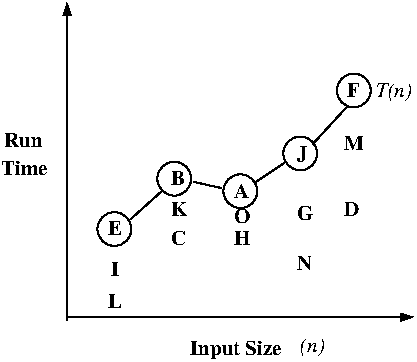
  • The road from actual running time to asymptotic worst-case time complexity -- necessary lies (or rather, abstractions):

    		C(x)		T(n)		T(n)		O(g(n))
    Actual		Abstract		(Exact)		Worst-Case		Asymptotic
    Running	----->	Running	----->	Time	----->	Time	----->	Worst-Case
    Time		Time		Complexity		Complexity		Time
    								Complexity
    		Instruction		Input Size		Worst-Case		Asymptotic
    		Counts				Selection		Notation

  • Let's look at various concepts and techniques mentioned above in more detail.
  • Counting instructions

    

    • Motivated by the need for "machine" (computer hardware / operating system, programming language) -independent measure of algorithm efficiency.
    • Basic instructions in a program can have a wide range of running times. Can indicate this in an analysis by assigning a separate constant for the running time of each kind of instruction; is accurate, but very cumbersome.
    • We will assume that each kind of basic instruction runs in 1 time unit. Is not accurate but does simplify analyses; moreover, can be justified by our ultimate focus on asymptotic time complexity.
    • We will assume a RAM model of memory in which all stored elements are accessible in 1 time unit. Is not accurate, as we ignore memory hierarchy; however, does simplify analyses.
  • Input size.

    

    • Motivated by the need to organize set of instruction-counts over the space of all inputs.
    • Assumes a "reasonable" encoding of inputs, e.g., numbers stored in binary (pages 1055-1057; see also Chapter 2, Garey and Johnson (1979)).
    • Isolate one or more parameters that describe amount of memory used to store input, e.g., length of a given list, the number of vertices in a given graph.
    • Hard to define formally; acquired informally via experience doing time complexity analyses.
    • We will assume where possible that we are dealing with small numbers in the input that fit inside a single computer-memory "word"; hence, the size of numbers in the input need not be a parameter in the input size.
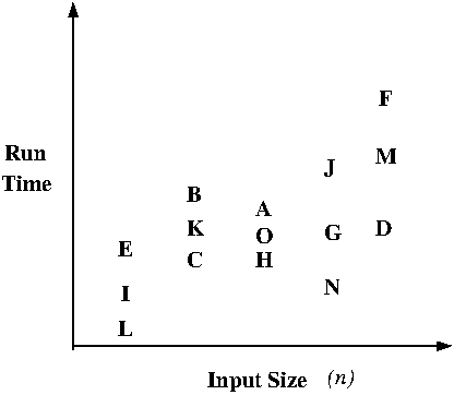
  • Time Complexity
    • Time complexity = instruction-count stated as function of input size.
    • Two general methods to deriving a time complexity function for an algorithm:
      • Compute counts for individual instructions and add together to derive function.
      • "Grow" function by starting at innermost level of nesting in algorithm and working outwards.

      Which method you use depends on the intricacy of the given algorithm.

    • Individual assignment statements count as a single instruction, regardless of the complexity of the expression on the right-hand size.
    • Each type of control-structure has its own rule for counting instructions.
    • while-loop rule: #iter(body + 1) + 1
      • The first "1" in the expression is for the evaluation of the loop-execution condition (to TRUE) for the executions of the loop body, and the second "1" is for the final evaluation of the loop-execution condition (to FALSE) when the loop terminates.
    • Example: while-loop.
    • Example: Example Algorithms #1 and #2 (tc_examples_1.txt)
    • for-loop rule: #iter(body + 2) + 2
      • The first "2" in the expression is for the evaluation of the loop-execution condition (to TRUE) and increment of the index variable for the executions of the loop body, and the second "2" is for the initialization of the index variable before the loop starts and the final evaluation of the loop-execution condition (to FALSE) when the loop terminates.
      • This is very clearly seen if you rewrite a for-loop as the equivalent while-loop.
    • Example: for-loop.
    • Example: Doubly-nested for-loop: the selection sort algorithm (tc_sorting.txt)
  • Worst-Case Time Complexity

    

    • Programs involving loops and simple statements naturally give time complexity functions such that every input of a particular size runs in the same time; unfortunately, once we allow arbitrary while and if-then-else statements, different inputs of the same size may run in different times, e,g., sorting algorithms on sorted and unsorted lists of the same length.
    • Need to summarize set of running times for each input size s by a single number. There are three options:
      1. Best-case, e.g., lowest running time over all inputs of size s; easy to compute but not that useful in practice.
      2. Average-case, e.g., average running time relative to some probability distribution over all inputs of size s; useful in practice but hard to compute.
      3. Worst-case, e.g., highest running time over all inputs of size s; easy to compute and useful in practice -- moreover, simplifies analyses (see rule for if-then-else below).
    • Worst-case time complexity functions are both useful and usable; hence, are most commonly in practice.
    • if-then-else-statement rule: max(if-body, else-body) + 1
    • Example: Two analyses of Example Algorithm #3 (tc_examples_1.txt)
    • Example: the linear and binary search algorithms (tc_searching.txt)
    • Example: the bubble and insertion sort algorithms (tc_sorting.txt)
  • Asymptotic notation

    

    • Used to smooth and simplify time complexity functions; assumes input size goes out to infinity, and that simplification can be stated in terms of "essential" behavior of function in the limit.
    • What makes a function g(n)) a useful and smooth upper bound of a time complexity function function g(n) ?
      • g(n) upper-bounds f(n):
        f(n) <= g(n) for all n > 0.

      • g(n) upper-bounds f(n) after initial "bumpy" portion:
        f(n) <= g(n) for all n > n0 for some n0 >= 0.

      • g(n) upper-bounds f(n) after initial "bumpy" portion under arbitrary machine model:
        f(n) <= c * g(n) for all n > n0 for some c > 0 and n0 >= 0.

        This allows (to a degree) for instructions whose running-times differ by a constant multiplicative factor on different machines.

      Note that we have re-derived the definition of big-Oh asymptotic upper-bound notation by combining the mathematical requirements of a useful smoothing function.
    • Asymptotic upper bounds: Big-Oh notation (O(g(n))).
      • Example: T(n) = 3n^2 + 4n + 5 is O(n^2) (big_Oh.txt)
      • One could derive the required constant c by fancy algebra; I prefer to set c to the sum of the positive coefficients -- it's very dirty but it's also quick.
      • Example: T(n) = 3n^2 + 4n + 5 is not O(n) (big_Oh.txt)
      • Try to avoid ludicrously loose upper bounds.
      • Example: T(n) = 2n is O(n^57)
      • Relationship between informal "T(n) is O(g(n))" definition and "O(g(n)) as the set of all g(n)-upper-bounded functions" definition given in textbook; keep the latter in mind, but the former is colloquial CS usage. May stem from algorithm-centric and math-centric views of asymptotic notation, respectively.
    • Asymptotic lower bounds: Omega notation (OMEGA(g(n))).
      • Example: T(n) = 3n^2 + 4n + 5 is OMEGA(n^2) (big_OMEGA.txt)
      • Example: T(n) = 3n^2 + 4n + 5 is not OMEGA(n^3) (big_OMEGA.txt)
      • Try to avoid ludicrously loose lower bounds.
      • Example: T(n) = 2n^57 is OMEGA(n)
    • Asymptotic exact bounds: Theta notation (THETA(g(n))).

Thursday, January 16 (Lecture #3)
[Section 3.1; Class Notes]

• Background: Time Complexity (Cont'd)
  • Asymptotic notation (Cont'd)
    • Three caveats on using asymptotic notation:
      1. How you interpret asymptotic notation depends on how the function T(n) was derived. If T(n) is an exact value for all inputs of a size n, then can say T(n) = O(g(n)) (OMEGA(g(n))) [THETA(g(n))] means "the running time is upper (lower) [exactly] bounded by g(n)"; however, if T(n) is merely an upper bound on the running time (as has been the case in our most recent examples), must be more careful in interpreting OMEGA and THETA statements.
      2. Though it is in a sense an abuse of notation, you will frequently see O(1) or THETA(1) used to indicate an unspecified constant in various expressions.
      3. The rules about combining separate asymptotic-notation expressions are tricky; be VERY careful if you ever do this in your math -- it might be better off to write out the full constant-bounds and work with those, so you don't make mistakes.
    • Guidelines for deriving asymptotic worst-case time complexity functions (non-recursive algorithms)
      • If you have a worst-case time complexity function on hand, the leading term (minus coefficient) is usually the asymptotic worst-case time complexity function.
      • Example: Though the selection, bubble, and insertion sort algorithms run in T(n) = 4n^2 - 2, T(n) = 7n^2 - 3n + 2, and T(n) = 3n^2 - 1 time, respectively, all of these algorithms run in O(n^2) time.
      • As constants associated with different loops and different numbers of embedded simple statements vanish into the leading constant c in the definition of asymptotic notation, can often derive a near-optimal asymptotic worst-case time complexity function by simply multiplying out the number of iterations for each loop in the deepest chain of nested loops.
      • Example: As both the insertion and selection sort algorithms consist of a pair of nested loops, each of which has at most n iterations, both algorithms run in O(n * n) = O(n^2) time.
      • The usual way to handle nested if-then-else statements is to assume the largest sub-case always executes. However, if you have a function describing how often the conditional is true, you may be able to do better, e,g., derivation of O(|V| + |E|) time complexity for breadth-first graph traversal algorithm (see also the second analysis of Example Algorithm #3).
  • Parameterized time-complexity expressions
    • If you are ever confronted with an algorithm which uses operations of unspecified time complexity, build a parameterized time-complexity expression and solve this expression as necessary when you are given the time complexities of those operations.
    • Example: Parameterized versions of Example Algorithms #1 and #2 (tc_param.txt)
    • A particularly useful variant of such expressions are asymptotic worst-case parameterized time-complexity expressions, i.e., simplified big-Oh worst-case versions of parameterized time-complexity expressions.
      • Very useful if algorithm incorporates conditional and/or conditional-loop statements.
      • Derive using the same techniques as you use to derive asymptotic worst-case time complexity expressions modulo the inclusion of variable-terms for unknown operation time complexities.
      • If the term X indicating the execution of the deepest nested loop statements is the same as the term in front of one of unknown-procedure runtimes then ignore X, e.g., O(n^2T(P1) + nT(P2) + n^2) => O(n^2T(P1) + nT(P2)).
      • If the term X indicating the execution of the deepest nested loop statements is greater than the term in front of one of unknown-procedure runtimes then leave X in the expression, e.g., O(n^2T(P1) + nT(P2) + n^3) => O(n^2T(P1) + nT(P2) + n^3).
    • Example: The asymptotic worst-case parameterized time-complexity expressions for Example Algorithms #1 and #2 in the previous example are O(nT(P1)) and O(n^2T(P2) + nT(P1)), respectively.
    • Very nice when you are evaluating an algorithm that uses a set of operations and that set of operations is supported (albeit with different time complexities) by each of a set of data structures -- one derives the parameterized "generic" time complexity for the algorithm and then you derive the time complexity relative to each of the data structures (by filling in the time complexities for the operations relative to that data structure).
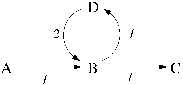
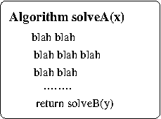
    • Also very nice for relating two problems. Suppose a problem P1 can be solved by an efficient, i.e, (asymptotic worst-case) polynomial time, algorithm that invokes a procedure that solves instances of a problem P2, i.e.,

      		    P1(n):
      		      blah blah blah
      		      x = P2(n)
      		      blah blah blah
      		      output z
      		    

      This has several implications:
      • If P2 is efficiently solvable than so is P1 (simply substitute the efficient algorithm for P2 into the algorithm for P1 described above) .
      • If P1 is not efficiently solvable than neither is P2 (if P2 was efficiently solvable, you could substitute that algorithm into the algorithm above for P1 to create an efficient algorithm for P1, which is a contradiction).

      The former is the reason why we create efficient libraries of commonly-called algorithms; as we shall see in the final section of this course, the latter is the basis for showing that a problem does not have an efficient algorithm.

• Potential exam questions
• Algorithm Design Techniques
  • Combinatorial optimization problems redux
    • Each solution associated with an instance of a combinatorial optimization problem has a cost, and we want the solutions of optimal (min/max) cost over the whole solution space.
      • Any time you have a problem of the form "Find the best X" where X is some discrete structure, chances are you're dealing with a combinatorial optimization problem.
    • Distinguish several types of solutions:
      • Candidate solutions = all possible solutions to the instance, e,g., all possible edge-sequences of a given graph that start with vertex u and end with vertex v.
      • Viable solutions = all potentially optimal candidate solutions, e.g., all edge-sequences of a given graph that are paths between vertices u and v.
      • Optimal solutions = those viable solutions that have optimal value relative to the cost function over the set of viable solutions, e.g., all paths in a given graph between vertices u and v that have the smallest number of edges over the space of all such paths.
    • Each such problem instance has a combinatorial, i.e., exponential in instance size, candidate (and often viable) solution space -- the job of an algorithm is to to find the optimal solutions in this space (of which there will always be at least one).
    • Sometimes, you can't generate viable solutions -- you have to generate all candidate solutions and check viability along the way.
    • Example: The 0/1 Knapsack problem
      • Candidate solutions = subsets of U.
      • Viable solutions = subsets of U whose summed size is <= B.
      • Optimal solutions = subsets of U whose summed size is <=B and whose summed value is maximum over the space of viable solutions.
      • Each subset U' can be modeled as a binary vector of length |U| (v_i = 1 (0) => item i is (not) in U'); hence, there are 2^{|U|} candidate solutions for any instance of 0/1 Knapsack.
    • Sometimes, you can generate viable solutions up front -- this depends in part on your ingenuity.
    • Example: The Longest Common Subsequence problem

      Longest common subsequence (LCS)
      Input: Two strings s, s' over an alphabet Sigma.
      Output: All strings s'' over Sigma such that s'' is a subsequence of both s and s' and the length of s'' is of is maximized over the solution space.

      • Candidate solutions = all possible strings over alphabet Sigma of length <= min(|s|,|s'|).
      • Viable solutions = all subsequences of the shorter given string.
      • Optimal solutions = all subsequences of the shorter given string that are also subsequences of the longer given string and have the maximum length over the space of viable solutions.
      • Each subsequence s'' can be modeled as a binary vector of length min(|s|,|s'|) (v_i = 1 (0) => symbol i is (not) included in the subsequence); hence, there are O(2^{min(|s|,|s'|)}) viable solutions for any instance of LCS (note that this worst case only occurs if each symbol in s and s' only occurs once).
    • Sometimes even the set of viable solutions is dauntingly large (like, REALLY large).
    • Example: The Minimum Spanning Tree problem
      Minimum spanning tree (MST)
      Input: An edge-weighted graph G = (V, E, w).
      Output: All spanning trees T of G, i.e., trees that connect all vertices in G, such that the sum of the weights of the edges in T is minimized over the solution space.
      • Candidate solutions = all (|V| - 1)-sized subsets of the edges of G.
      • Viable solutions = all (|V| - 1)-sized subsets of the edges of G that are spanning trees of G.
      • Optimal solutions = all spanning trees of G that have minimum summed edge-weight over the space of viable solutions.
      • By Cayley's Theorem, a graph G = (V, E) has O(|V|^{|V| - 2}) spanning trees (the worst case here is when G is a complete graph); hence, there are O(|V|^{|V| - 2}) viable solutions for any instance of MST.
    • Can solve combinatorial optimization problems by looking at all (candidate/viable) solution and saving those of the optimal cost (which we can determine on the fly by saving those solutions with the best cost we've seen so far at any point in the enumeration of all solutions).
    • This is inherently inefficient given the exponential sizes of the (candidate/viable) solution spaces involved. Can we do better?
      • We most certainly can. Consider MST; though the set of viable solutions for each instance of MST is potentially exponentially large, we can solve all instances of MST in low-order polynomial time.
      • How good we can do algorithm-wise depends on how much of the (candidate/viable) solution space our algorithm can ignore. Over the next 8 lectures, we'll examine a set of techniques for doing this whose applicability depend on some fairly simple properties of problem solution-spaces.
  • Combinatorial Solution-Space Trees (Sections 9.1-9.7, B&B)
    • The most basic approach to solving combinatorial optimization problems in which we are interested in finding a subset SS' of a given set SS such that c(SS') is optimal relative to some solution-evaluation function c().
    • As a first step, simplify generation of solutions for a problem instance by using a combinatorial solution-space tree (CST).
      • In such a tree, internal nodes are partial solutions and the full solutions labeling the leaves comprise the solution space.
      • The simplest such trees are binary, and each of the |SS| levels in the tree effectively decides whether or not to add a particular item in SS to the solution
    • Example: A CST for an instance of 0/1 Knapsack in which SS = U = {X, Y, Z} and |SS| = |U| = 3:

      

Tuesday, January 21 (Lecture #4)
[Class Notes]

• Algorithm Design Techniques (Cont'd)
  • Combinatorial Solution-Space Trees (Cont'd)
    • One can vary the items added at each CST level to construct different types of solutions for different problems.
    • Example: A CST for an instance (s = ABAACA, s' = ADC) of Longest common subsequence in which SS = {1, 2, 3}, i.e., positions in the shorter given string (in this case, s') and |SS| = |s'| = 3:

      

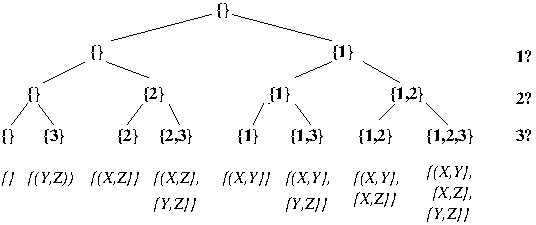
    • Example: A CST for an instance (I = {X, Y, Z}, S = {{X, Y}, {X, Z}, {Y, Z}}) of Set cover (see Assignment #1) in which SS = {1, 2, 3}, i.e., the numbers of the subsets of I in S, and |SS| = |S| = 3:

      

    • Can traverse such a tree and examine all of its leaves using depth-first search (DFS) or breadth-first search (BFS). Only those leaves corresponding to viable solutions are important.
    • Example: Viability conditions for 0/1 Knapsack, LCS, and MST.
      • Do items in partial solution fit in knapsack? (0/1 Knapsack)
      • Is partial solution string a subsequence of both given sequences? (LCS)
      • Do edges in partial solution form a forest? (MST)
    • As a second step, decrease space requirements by operating on an implicit CST, i.e., generate tree nodes as necessary during traversal.
    • ALGORITHM: DFS-based traversal of implicit CST (minimization version) [ASSIGNMENT #1]

       1. DFS-I(i, sol)
       2.    if (i == n + 1)
       3.       if (viable (sol))
       4.           return(cost(sol))
       5.       else
       6.           return(INFINITY)
       7.   else
       8.       return(min(DFS-I(i + 1, sol),
       9.                  DFS-I(i + 1, sol U item[i])))
      

      • Initial call: DFS-I(1, empty set)
      • Note that n is the number of items in the set in the instance; hence "i == n + 1" means that you have reached a leaf in the CST.
    • ALGORITHM: BFS-based traversal of implicit CST (minimization version).

       1. BFS-I()
       2.    Q = {(1, empty set)}
       3.    best = INFINITY
       4.    while not empty(Q)
       5.      (i, sol) = pop(Q)
       6.      if (i == n + 1)
       7.         if (viable(sol))
       8.            best = min(best, cost(sol))
       9.      else
      10.         push(Q,(i + 1, sol))
      11.         push(Q,(i + 1, sol U item[i]))
      12.    return(best)
      

    • Modifications:
      • To make the above work for maximization problems, change min to max and INFINITY to -INFINITY.
      • To obtain optimal solutions, the simplest way is to run a second tree-traversal that takes the optimal cost produced previously as a parameter and stores / prints all viable solutions with that cost.
    • Example: Execution of DFS-based traversal of implicit CST for 0/1-Knapsack when U = {X,Y,Z}, s(X) = 4, s(Y) = 2, s(Z) = 1, v(X) = 4, v(Y) = 5, v(Z) = 3, and B = 4:

      

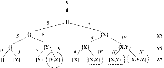
      Note that optimal leaf-solutions are circled and non-viable leaf-solutions are enclosed in dashed boxes.

    • INTERLUDE: A look at the mechanics of Assignment #1.
    • This is all well and good; however, we are still looking at every node in the tree, and as this tree is of exponential size, our algorithm runs in exponential time. Can we do better? Yes we can!
    • As a third step, where possible, use information about partial solution viability and potential optimality to terminate search of unfeasible subtrees of the CST (dynamic pruning).
      • Traditionally, DFS + dynamic pruning is known as backtracking and BFS + dynamic pruning is known as branch and bound.
      • Dynamic pruning works in CST because all "full" candidate solutions that incorporate a particular particular partial solution are leaves in the subtree rooted at the node corresponding to that partial solution; hence, non-viability / non-potential-optimality of a partial solution implies the non-viability / non-potential-optimality of all solutions in the subtree rooted at the node corresponding to that partial solution!
    • Example: Potential optimality conditions for 0/1 Knapsack, LCS, and MST.
      • Does sum of values of items in partial solution plus sum of values of all remaining items that could be added exceed the value of the best solution seen so far? (0/1 Knapsack)
      • Does the length of the partial solution string plus the length of the string of all remaining characters that could be added exceed the length of the best solution string seen so far? (LCS)
      • Is the sum of the weights of the edges in the partial solution less than the cost of the best solution found so far? (MST)
    • ALGORITHM: DFS-based traversal of implicit CST + dynamic pruning (minimization version).

       1. DFS-IP(i, sol, best)
       2.    if (not viable(sol)) or (best < cost(sol))
       3.       return(INFINITY)
       4.    else if (i == n + 1)
       5.       best = min(best, cost(sol))
       6.       return(cost(sol))
       7.    else
       8.       return(min(DFS-IP(i + 1, sol, best),
       9.                  DFS-IP(i + 1, sol U item[i], best)))
      

      • Initial call: DFS-IP(1, empty set, BEST) where BEST is an object encoding the integer INFINITY.
      • Note that variable BEST is passed by reference, e.g., it is a pointer to an integer; if it is passed by value, the value of BEST is not saved from any of the leaf-evaluations.
    • ALGORITHM: BFS-based traversal of implicit CST + dynamic pruning (minimization version).

       1. BFS-IP()
       2.    Q = {(1, empty set)}
       3.    best = INFINITY
       4.    while not empty(Q)
       5.       (i, sol) = pop(Q)
       6.       if (viable(sol) and (cost(sol) < best))
       7.	     if (i == n + 1)
       8.             best = min(best, cost(sol))
       9.          else
      10.             push(Q,(i + 1, sol))
      11.             push(Q,(i + 1, sol U item[i]))
      12.    return(best)
      

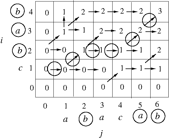
    • Example: Execution of DFS-based traversal of implicit CST for 0/1-Knapsack with dynamic pruning based on non-viability when U = {X,Y,Z}, s(X) = 1, s(Y) = 3, s(Z) = 2, v(X) = 1, v(Y) = 4, v(Z) = 2, and B = 3:

      

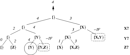
      Note that optimal solutions are circled and non-viable solutions are enclosed in dashed boxes.

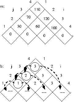
    • Example: Execution of DFS-based traversal of implicit CST for 0/1-Knapsack with dynamic pruning based on both non-viability and non-potential optimality when U = {X,Y,Z}, s(X) = 1, s(Y) = 3, s(Z) = 2, v(X) = 1, v(Y) = 4, v(Z) = 2, and B = 3:

      

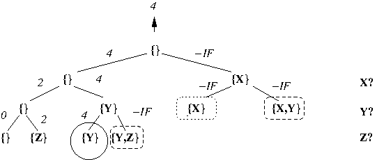
      Note that optimal solutions are circled and non-viable (non-potential optimal) solutions are enclosed in dashed (dotted) boxes.

    • Such tricks can (but may not always) drastically reduce actual running times for CST traversal.
    • Food for Thought:
      1. Can we do better in practice runtime-wise if we only require one optimal solution? How about in the worst case?
      2. Can we do better in practice runtime-wise if we require all optimal solutions? How about in the worst case?
  • Potential exam questions

Thursday, January 23 (Lecture #5)
[Sections 2.3.1, 4.2, and 15.3-4; Class Notes]

• Algorithm Design Techniques (Cont'd)
  • The CST approach to solving combinatorial optimization problems assumes nothing about the structure of the solution space for an instance. If we did have such knowledge, can we do better?
  • There are other types of computation trees besides CST. There are, for example, the trees associated with recursive computations, in which nodes represent individual recursive algorithm calls on subproblems of smaller size. Such a recursive-call tree is also called a recursive decomposition.
  • Characteristics of recursive decomposition:
    • Can decompose instance of problem into smaller instance of the same problem, i.e., subproblems.
    • At any point in the computation, may be several choices for decomposition.
  • Problems that are solvable by recursive decomposition have the optimal substructure property, i.e, an optimal solution for an instance of the problem can be constructed using optimal solutions for instances of that problem that are of smaller size (subproblems)..
  • Our remaining algorithm design techniques will be applicable if a problem's recursive decomposition satisfies additional properties.
  • Divide-and-Conquer (D&C)
    • Applies if a problem has recursive decomposition in which each subproblem occurs only once, i.e., the subproblems do not repeat.
    • Will typically only be efficient if the depth of recursion is logarithmically bounded, thus ensuring that the total number of recursive calls is polynomially bounded.
    • Example: Binary search in a sorted list
      • Look at midpoint in current list; if wanted element is not there, repeat midpoint search on lower (upper) half sublist if wanted element is less (greater) than the midpoint.
      • Each sublist is searched only once; moreover, can only halve a list of n elements log_2 n times.
      • Can be done in O(log_2 n) time.
    • Example: Merge sort (Section 2.3.1)
      • Recursively halve a list until sublists have single elements, and on return, merge sorted sublists in linear time.
      • Each sublist is sorted only once; moreover, can only halve a list of n elements log_2 n times.
      • Can be done in O(n log_2 n) time.
    • Example: Strassen's matrix multiplication algorithm (Section 4.2)
      • Can rephrase multiplication of two n x n matrices by recursively decomposing each matrix into four n/2 x n/2 submatrices and intricately multiplying and adding these submatrices.
      • Each submatrix is multiplied only once; moreover, can only halve an n x n matrix log_2 n times.
      • This still requires O(n^3) but if we apply a more intricate still submatrix multiplication / addition scheme due to Strassen, we get a runtime of O(n^{log_2 7}).
  • The relationship between CST and Divide-and-Conquer algorithms:

    				Optimal
    			      Substructure?
    		             /          \
    			    / YES        \ NO
    	                   /              \
    	                 D&C              CST
    	      

  • How can we exploit the optimal substructure problem if subproblems are repeated?
  • Dynamic Programming
    • Applies if a problem has a recursive decomposition and the number of distinct problems is bounded and can be organized in some n-dimensional table.
    • Example: Computing Fibonacci numbers
      • Recurrence (recursive + base cases)
        • Fib(i) = ith Fibonacci number, i >= 1
        • Fib(i) = Fib(i - 1) + Fib(i -2) for i > 2.
        • Fib(1) = Fib(2) = 1
      • ALGORITHM: Fibonacci numbers (Recursive)

         1. FibR(n)
         2.    if ((n == 1) || (n == 2))
         3.       return(1)
         4.    else
         5.       return(FibR(n - 1) + FibR(n - 2))
        

      • Recursive-calls tree: 2^{n/2} - 1 <= Tree Size <= 2^{n} - 1
      • The problem here is that subproblems are being repeated; perhaps the recursive algorithm can keep track of what subproblems have been solved by storing those values in a table and look these up as necessary? An algorithm that does this is called a memoized algorithm.
      • ALGORITHM: Fibonacci Numbers (Memoized (Recursive))

         1. InitFibT(n,FibT)
         2.    Allocate n-element table and assign to FibT
         3.    FibT[1] = FibT[2] = 1
         4.    for (i = 3; i <= n; i++)
         5.       FibT[i] = INFINITY
        
         6. FibM(n, FibT)
         7.    if (FibT[n] == INFINITY)
         8.       FibT[n] = FibM(n - 1, FibT) + 
         9.                 FibM(n - 2, FibT)
        10. return(FibT[n])
        

      • This table idea was pretty neat. In fact, do we really need the recursion anymore? Let's just fill out the table!
      • ALGORITHM: Fibonacci Numbers (Dynamic programming (Iterative))

         1. FibI(n)
         2.    if ((n == 1) || (n== 2))
         3.       return(1)
         4.    else
         5.       Allocate n-element table FibT
         6.       FibT[1] = FibT[2] = 1
         7.       for (i = 3; i <= n; i++)
         8.           FibT[i] = FibT[i - 1] + FibT[i - 2]
         9.       return(FibT[n])
        

    • If we are lucky, there are a polynomial number of distinct subproblems. If we are really lucky, we can use the recurrence to solve these subproblems in a "bottom up" rather than a "top down fashion", solving the smallest subproblems first and solving progressively larger subproblems until we solve the original problem instance.
    • Dynamic programming (DP) => table-driven, bottom-up recursive decomposition algorithms!
    • The Dynamic Programming Cookbook:
      • Step 1: Find a recurrence / recursive decomposition for the problem of interest; this includes approprtiately defining the problem of interest.
        • The subproblems typically ask for the cost of an optimal solution to a subproblem.
      • Step 2: Lay out the distinct subproblems in a table.
      • Step 3: Fill in the base-case values in the table.
      • Step 4: Run the recurrence "in reverse" / in a bottom-up fashion, using smaller solved subproblems to solve larger subproblems, until the table is filled in.
        • This fillin typically includes information about the choice(s) made in solving a subproblem (backpointers) that is used in Step 5.
      • Step 5: Use traceback on backpointers starting from the optimal-cost table entry for the original subproblem of interest to reconstruct one or more optimal solutions for that problem.
    • Example: DP algorithm for Longest Common Subsequence (LCS)
      • Recursive decomposition
        • Given strings s and s' over some alphabet, D(i,j) = length of longest common subsequence of first i characters of s and first j characters of s'.
        • Two recursive cases:
          1. ith character of s and jth character of s' are the same.
          2. jth character of s and jth character of s' are different.
      • Recurrence (recursive + base cases)
        • Case 1: D(i,j) = D(i - 1, j - 1) + 1 for i, j > 0
        • Case 2: D(i,j) = max(D(i, j - 1), D(i - 1, j)) for i, j > 0
        • D(i,0) = D(0,j) = 0 for i, j >= 0
      • Matrix fill-in (including backpointers) for deriving length of longest common subsequence.
        • Rectangular (m + 1) x (n + 1) matrix; fill-in proceeds from cell (1,1) row-wise, column-wise, or anti-diagonal-wise.
        • Fill-in of an individual cell involves consulting filled-in cells in the 3-cell "overhang" to left and above of that cell.
        • Backpointer cells have value 1, 2, or 3 depending on which recursive (sub)case was invoked.
      • Derivation of an LCS involves matrix-fill in get the length of a longest common subsequence followed by traceback from cell D(|s|,|s'|) for deriving a longest common subsequence.

Tuesday, January 28 (Lecture #6)
[Section 15.4]

• Algorithm Design Techniques (Cont'd)
  • Dynamic Programming (Cont'd)
    • Example: DP algorithm for Longest Common Subsequence (LCS) (Cont'd)
      • Example: LCS of s = cbab and s' = abacab

        

        Observe that the reconstructed LCS is bab (matching characters in s and s' as well as the traceback path to derive this subsequence are indicated by circled elements).

      • Example: LCS of s = ABCBDAB and s' = BDCABA (page 395).
      • DP algorithm (table fill-in (page 394) + traceback (page 395))
      • Time complexity of matrix fill-in: (# cells) x (#choices per cell) x (max # subproblems per choice) = (m + 1)(n + 1) x 2 x 2 = O(mn)
      • Time complexity of traceback = O(m + n) [longest possible backpointer path from D[|s|,|s'|] to D[0,0]].
      • Space complexity: # cells = (((m + 1) x (n + 1)) = O(mn)
      • Food for thought:
        1. How does the above change if we want to enumerate all possible LCS of s and s'?
        2. Can we do better spacewise if all we want is the length of an LCS of s and s'?
        3. Can we do better spacewise when obtaining a single LCS of s and s'?
        4. How does the above change if there are different degrees of symbol identity, e.g., identical a's are worth more than identical b's or c's?
        5. How does the above change if we want to compute longest common substrings?
      • INTERLUDE: A look at the mechanics of Assignment #2.

Thursday, January 30 (Lecture #7)
[Sections 15.2-3]

• Algorithm Design Techniques (Cont'd)
  • Dynamic Programming (Cont'd)
    • Example: DP algorithm for Matrix Chain Parenthesization (MCP)
      • Review of 2-matrix multiplication: O(n^3) time (n = max matrix dimension)
        • Multiplication of (n x l) matrix M1 and (l x m) matrix M2 requires n * l * m multiplications and produces an n x m matrix.
      • 3-matrix multiplication: Parenthesization of matrix "chain" for 2-matrix multiplication can drastically affect the number of individual element multiplications.
      • Example: Given matrices M1 (2 x 5), M2 (5 x 100), and M3 (100 x 2), (M1 * M2) * M3 uses (2 * 5 * 100) + (2 * 100 * 2) = 1400 multiplication operations but (M1 * (M2 * M3) uses (2 * 5 * 2) + (5 * 100 * 2) = 1020 multiplication operations.
      • Recursive decomposition
        • m(i,j) = minimum number of element multiplications required to multiply matrices i through j in the given chain.
        • Let the dimensions of our n matrices be encoded in in an (n+1)-length array p with index starting at 0, where the dimensions of the ith matrix, 1 <= i <= n, are p[i-1] x p[i].
        • Value m(i, j) for i < j is the sum of the values of the best two-way split of matrix subsequence i through j plus the cost of multiplying the matrices produced by this split.
      • Recurrence (recursive + base cases)
        • m(i,j) = min_{i <= k < j} m(i,k) + m(k+1,j) + p[i-1]p[k][p[j] for i, j >= 1
        • m(i,i) = 0 for i >= 1
        • Note that this is the first recurrence we've seen that involves a non-constant number of subproblem decomposition choices.
      • Matrix fill-in (including backpointers) for deriving minimum number of multiplications relative to optimal matrix chain parenthesization. subsequence.
        • Ragged-bottom pyramid / B2 bomber shape matrix; fill-in proceeds from left to right in ascending rows.
        • Fill-in of an individual cell involves consulting filled-in cells in the "boomerang" hanging off that cell.
        • Backpointer matrix cells have value k at which matrix sequence i .. j split into matrix subsequences i .. k and (k + 1) .. j.
        Traceback is initiated from cell m(1,n) for an for an optimal matrix parenthesization.
      • Example: Optimal parenthesization of matrix sequence M1 (2 x 3), M2 (3 x 5), M3 (5 x 4), and M4 (4 x 5).

        

        Full value and backpointer computations for matrices m and b are given here. Observe that the above yields the optimal parenthesization (((M1 M2) M3) M4).
      • Example: Optimal parenthesization of matrix sequence M1 (30 x 35), M2 (35 x 15), M3 (15 x 5), M4 (5 x 10), M5 (10 x 20), and M6 (20 x 25) (page 376).
      • DP algorithm (table fill-in (page 375) + traceback (page 377))
      • Time complexity of matrix fill-in: (# cells) x (#choices per cell) x (max # subproblems per choice) = (n(n - 1)/2) x (n - 1) x 2 = O(n^3).
      • Time complexity of traceback = n - 1 = O(n) [longest possible backpointer path from D[1,n|] to base-case entry].
      • Space complexity: # cells = n(n - 1)/2 = O(n^2)
      • Food for thought:
        1. How does the above change if we want to enumerate all possible MCP of given matrix-chain?
        2. Can we do better spacewise when obtaining a single MCP of a given matrix-chain?
        3. Can we do better spacewise if all we want is the cost of a MCP of a given matrix-chain?
    • Another important characteristic of problems whose optimal substructure can be exploited by dynamic programming (and indeed by divide-and-conquer and greedy algorithms as well) is subproblem independence, i.e., solutions to subproblems do not share resources. This is important because subproblem solutions can only be combined if they are independent.
    • Example: The existence (impossibility) of dynamic programming algorithms for the unweighted shortest (longest) simple path problems in directed graphs (pp. 381-384).
      • Recall that in a simple path, vertices cannot repeat.
      • USSP has the optimal substructure property.
        • Consider a shortest path p between any two vertices u and v incorporating an intermediate vertex w (which may be u or v); this can be decomposed into subpaths p1 and p2 between u/w and w/v, respectively.
        • If p is a shortest path between u to v then then p1 must be a shortest path between u and w (proof by contradiction: if there was a shorter path p` between u and w, it could be combined with p2 to create a path shorter than p, which contradicts the optimality of p).
        • An analogous argumnent establishes the optimality of p2.
        • This recursive decomposition is the basis of a shortest-path algorithm we will examine later in this course.
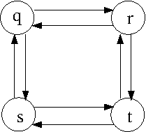
      • ULSP does not have the optimal substructure property.
        • Consider the following graph G:

          

          Observe that the longest simple path between q and t is q-r-t, but the longest simple path between q and r (q-s-t-r) cannot be combined with the longest simple path from r to t (r-q-s-t) to get the longest simple path from q to t because vertices repeat in these two paths.
        • Unlike USSP, subproblems in ULSP are not independent, as they share resources (in this case vertices) and cannot be patched together to create solutions to larger problems.
      • ULSP does not have the optimal substrtucture property and hence does not have cool DP or Divide-and-Conquer algorithms; however, might there be another route to polynomial-time solvability for ULSP? As we shall see later in this course, the answer to this question is "probably not".

Tuesday, February 4

• In-class Exam #1 Notes
  I've finished making up the first in-class exam. The exam will be closed-book and written in-class on paper (please bring your own pens). It will be 75 minutes long and has a total of 50 marks (this is not coincidental; I have tried to make the number of marks for a question approximately equal to the number of minutes it should take you to do it in the best case). The exam will cover material in all course lectures up to and including Lecture #8 (Topics 2-4 in the potential exam question list). There will be four questions:
  1. Time complexity I [Topic 2] (3 parts / 9 marks)
  2. Time complexity II [Topic 2] (3 parts / 9 marks)
  3. Algorithm Design Techniques I [Topic 3] (2 parts / 20 marks)
  4. Algorithm Design Techniques II [Topic 4] (1 part / 12 marks)

  I hope the above helps, and I wish you all the best of luck with this exam.

Tuesday, February 4 (Lecture #8)
[Section 15.2; Class Notes]

• Algorithm Design Techniques (Cont'd)
  • Dynamic Programming (Cont'd)
    • Note that the dynamic programming algorithms we have seen so far are only useful because they have a polynomially-bounded number of subproblems -- this need not always be the case.
    • Example: DP algorithm for 0/1 Knapsack
      • Recursive decomposition
        • V(i,j) = summed of value of optimal knapsack load with size <= j, 0 <= j <= B, composed of selection from first i, 0 <= i <= |U|, items of U.
        • V(i,j) depends on whether or not item i can be added to a knapsack of size j.
      • Recurrence (recursive + base cases)
        • V(i,j) = max{V(i - 1,j), V(i - 1, j - s(u_i)) + v(u_i)}
          • First term: Cannot add item i to knapsack.
          • Second term: Can add item i to knapsack.
        • V(i,0) = V(0,j) = 0 (intuitively, both the knapsack of capacity 0 and the knapsack with 0 items to include in it have value 0); all other V(i,j) consulted by the recurrence are out of bounds of the table are assumed to have value -INFINITY.
      • Matrix fill-in (including backpointers) for deriving value of optimal knapsack.
        • Rectangular (|U| + 1) x (B + 1) matrix; fill-in proceeds from cell (1,1) row-wise, column-wise, or anti-diagonal-wise.
        • Fill-in of an individual cell involves consulting cell immediately above (V(i - 1,j)) and cell back one row to the left (V(i - 1, j - s(u_i))).
        • Backpointer matrix cells have value 1 or 2, depending on which recursive case was invoked.
      • Example: Optimal solution for 0/1 Knapsack when U = {u1,u2,u3}, s(u1) = 1, s(u2) = 3, s(u3) = 2, v(u1) = 1, v(u2) = 4, v(u3) = 2, and B = 4:

        

        Note that diagonal backpointers go back in the row and not necessarily to that backpointer's origin-cell. Observe that the above yields the optimal solution {u1,u2} with value 5.

      • Time complexity of matrix fill-in: (# cells) x (#choices per cell) x (max # subproblems per choice) = ((|U| + 1) x (B + 1)) x 2 x 1) = O(|U|B)
      • Time complexity of traceback = O(|U| + B) [longest possible backpointer path from V[|U|,B|] to V[0,0]].
      • Space complexity: # cells = ((|U| + 1) x (B + 1)) = O(|U|B)
      • Wait a minute ... this isn't a polynomial-time (or space) algorithm, because |U|B is not a polynomial of the input size (|U| + log B). What we actually have here is an exponential time algorithm!
      • Food for thought:
        1. How does the above change if we want to enumerate all possible optimal 0/1 Knapsaack solutions?
        2. Can we do better spacewise if all we want is the value of the optimal solution?
        3. Can we do better spacewise when obtaining a single optimal solution?
        4. Can we do better if we know that the value of B is bounded by some polynomial function in |U|?
      • Additional caveats:
        • DP is not necessarily better than CST!
          • CST for 0/1 Knapsack (DFS + pruning): O(2^{|U|}|U|) time, O(|U|) space.
          • DP for 0/1 Knapsack: O(|U|B) time and space.
          • CST always bettrer wrt space and better wrt time when |U| < log B.
        • There may be no "best" algorithm for a problem -- rather there are only algorithms that are the best relative to particular ranges of input-parameter values. It is therefore crucial for a human algorithm designer to both find those ranges of input-parameter values that characterize a given application AND reason about which algorithms are most appropriate for that application.
          • Sounds oddly like system requirements gathering and system architecture design in software engineering, yes?
          • Such activities are for now beyond automatic coding platforms like chatGPT and may point to roles only humans can play in future in algorithm and software system creation.
  • The relationship between CST, DP, and Divide-and-Conquer algorithms:

    				Optimal
    			      Substructure
    			          AND
                                  Independent
                                  Subproblems?
    		             /          \
    			    / YES        \ NO
    	                   /              \
    	              Repeated            CST
    		    Subproblems?
                       /            \
                      / YES          \ NO 
                     /                \
                   DP                  D&C
    	      

  • Potential exam questions

Thursday, February 6 (Lecture #9)
[Sections 16.1-16.2; Class Notes]

• Algorithm Design Techniques (Cont'd)
  • Dynamic programming and divide-and-conquer algorithms have enabled us to make many apparently difficult problems solvable in low-order polynomial time. Can we do still better? In certain cases, it seems that we can.
    • Consider binary search; it is a particularly interesting example of a D&C algorithm in which there is, at each point in the computation, at most 1 choice and 1 subproblem to be solved. In this case, the recursive computation collapses to a path of recursive calls from the "root" problem to a "leaf" subproblem.
    • The subproblem structure for binary search is unusually simple, in that a choice can be made before the subproblem is solved, i.e., the choice can be made in a top-down, locally optimal (greedy) manner. Compare this with other listed D&C and dynamic programming algorithms, which solve subproblems in a bottom-up manner and make choices only after all necessary subproblems have been solved.
    • As we we shall see, exploiting such greedy choices, while implementable succinctly in code, comes at the cost of increasingly complex proofs of correctness.
  • Greedy Algorithms
    • Example: The Activity Selection problem
      • Suppose we have set S = {a1, a2, ..., an} of activities that use a resourse such as a lecture room, where each activity ai has associated start and finish times si and fi such that 0 <= si < f1 < INFINITY.
        • We will assume that the activities in S are sorted in increasing order by finishing time, i.e., fi <= fj for i < j.
      • Two activities ai and aj are compatible if they do not overlap in time, i.e., fi <= sj.
      • The activity selection problem looks for the largest set of mutually compatible activities.
      • Example: Consider the following set of 11 activities (page 415):

        i  |   1   2   3   4   5   6   7   8   9  10  11
        ------------------------------------------------
        si |   1   3   0   5   3   5   6   8   8   2  12
        fi |   4   5   6   7   9   9  10  11  12  14  16
        

        The activities in the subset {a3, a9, a11} are all mutually compatible, but the largest such subset is {a1, a4, a8, a11}.
      • Recursive decomposition
        • Sij = the set of activities that start when or after ai finishes and finish before or when aj starts (we will assume "dummy" left and right endpoint activities a0 and a(n+1)).
        • c(i,j) = maximum number of mutually compatible activities in Sij.
          • Note that the value we need to solve the activity selection problem is c(0,n+1)!
        • Value c(i, j) for i < j is the sum of the values of the best two-way split of activity subsequence i through j plus 1 (that is, the best split at some solution-included activity k for i <= k < j).
      • Recurrence (recursive + base cases)
        • c(i,j) = max{i <= k < j} c(i,k) + c(k,j) + 1 if Sij is not empty.
        • c(i,j) = 0 if Sij is empty.
        • This looks an awful lot like the recurrence we derived for MCP, doesn't it?
      • Matrix fill-in (including backpointers) for deriving the optimal activity selection.
        • Ragged-bottom pyramid / B2 bomber shape matrix; fill-in proceeds from left to right in ascending rows.
        • Fill-in of an individual cell involves consulting filled-in cells in the "boomerang" hanging off that cell.
        • Backpointer matrix cells have value k at which matrix sequence i .. j split into activity subsequences i .. k and (k + 1) .. j.
      • Can we do better? In particular, do we have to evaluate all subproblem-pairs induced by a choice ak from S(i,j), or can we get away with a single ak-choice and subproblem?
        • It turns out that we can -- to get an optimal solution for S(i,j), greedily pick the activity am from S(i,j) with the earliest finishing time -- we are then left with the subproblem S(m,j)! (Theorem 16.1).
      • This gets even better -- note that instead of solving all S(i,j) in the bottom-up manner described above, we start with S(0,n+1) and solve directly in an iterative (and not recursive) top-down manner!
      • ALGORITHM: Activity Selection (Greedy (Recursive)) (page 419)
      • ALGORITHM: Activity Selection (Greedy (Iterative)) (page 423)

         1. ActSelGI(s, f)
         2.   n = s.length
         3.   A = {a1}
         4.   k = 1
         5.   for m = 2 to n do
         6.      if s(m) >= f(k) then
         7.         A = A u {am}
         8.         k = m
         9.   return A
        

      • Example: Derivation of an optimal activity selection in the example given above by the greedy algorithm (page 420).
      • Time AND space complexity (assuming we do not have to sort the activities in S by finishing time) = O(n).
      • Food for thought:
        1. Can we do better spacewise when obtaining a single optimal solution?
        2. Can we do better spacewise if all we want is the value of the optimal solution?
        3. How does the above change if we want to enumerate all possible optimal activity selections?
    • The Greedy Algorithm Cookbook [long form] (page 423)
      1. Determine the optimal structure of the problem, i.e., derive the recursive decomposition.
      2. Develop a recursive solution, i.e., derive the recurrence.
      3. Show that if we make the greedy choice then only one subproblem remains.
      4. Prove that it is always safe to make the greedy choice, i.e., that the greedy choice will always be part of some optimal solution.
      5. Develop a recursive algorithm that implements the greedy strategy.
      6. Convert the recursive algorithm to an iterative algorithm

Tuesday, February 11

• Instructor ill; lecture cancelled..

Thursday, February 13

• Instructor ill; lecture cancelled..

Tuesday, February 18 (Lecture #10)
[Sections 16.2 and 23.1-23.2; Class Notes]

• Algorithm Design Techniques (Cont'd)
  • The idea of greedy choice is seductive. In the absence of proofs of optimality, it underlies many heuristic algorithms whose performance is not gauranteed but have the virtues of being fast and simple, e.g., hill-climbing local search algorithms.
  • Are there easier ways than that explored in the previous lecture to derive and prove the optimality of greedy algorithms?
  • Greedy Algorithms (Cont'd)
    • Example: The Minimum Spanning Tree problem
      • DP algorithm.
        • Based on problems of the form P[i] = the cost of the minimum spanning forest for edge-weighted graph G that has i edges (note that what we ultimately want is P[|V| - 1]).
        • We can imagine a recurrence for P[i] in which we add all possible edges to solution-forests for P[i - 1] that connect two formerly distinct components in the forest and select those edges that result in minimum-cost forests on i edges. To do this, we need to associate the solution spanning-forests explicitly with P[i], i.e., we cannot reconstruct them after matrix fill-in by traversing backpointers.
        • The resulting recurrence has a double minimization over solution spanning-forests for P[i - 1] and edges that can be added to these forests, respectively.
      • Can we do better? In particular, do we have to evaluate all of the subproblems induced by all edge choices at each point, or can we get away with a single edge-choice and subproblem?
      • Consider the following very useful property of minimum spanning forests: Given such a forest for a graph G, each minimum-weight edge linking separate components in the forest must be in some minimum spanning tree for G (Theorem 23.1; see also Corollary 23.2). Such an edge is said to be safe.
      • What this means is that all we have to do is choose a safe edge and evaluate the resulting subproblem! This gets rid of the inner minimization over edges in the recurrence; moreover, as the choice of a safe edge always leads to some minimum spanning tree, we can also get rid of the outer minimization over spanning-forests.
      • ALGORITHM: Generic MST (page 626):

         1. MSTGen(G = (V,E,w))
         2.    F = (V, {})
         3.    for (i = 1; i <= |V| - 1; i++)
         4        Find a safe e in E for F = (V, E')
         5.       F = (V, E' u {e})
         6.    return F
        

      • Under appropriate selections of safe edges, this generic algorithm underlies both of the classic minimum spanning tree algorithms considered below.
      • Kruskal's algorithm (pages 631-633)
        • Start with trivial forest of G that just includes the vertices in V; add edges greedily, minimum-weight first, growing a minimum spanning forest that eventually coalesces into a minimum spanning tree for G.
        • ALGORITHM: Kruskal's MST Algorithm (page 631):

           1. MSTKruskal(G, w)
           2.    A = {}
           3.    for each vertex v in V do
           4.       MAKE-SET(v)
           5.    sort the edges in E in nondecreasing order by weight
           6.    for each edge in (u,v) taken in nondecreasing order by weight do
           7.        if FIND-SET(u) <> FIND-SET(v) then
           8.           A = A u {(u,v)}
           9.           UNION(u,v)
          10.    return(A)
          

        • Example: Example run of Kruskal's algorithm (pages 632-633) [Diagram]
        • Note that this a direct implementation of the generic MST algorithm above.
        • Running time
          = O(|V|(T(MAKE-SET)) + 2|E|(T(FIND-SET)) + |E|(T(UNION)) + SORT(|E|))
          = O(|V|(T(MAKE-SET)) + |E|(T(FIND-SET)) + |E|(T(UNION)) + |E| log |E|)
          = O(|V|(T(MAKE-SET)) + |E|(T(FIND-SET)) + |E|(T(UNION)) + |E| log |V|^2)
          = O(|V|(T(MAKE-SET)) + |E|(T(FIND-SET)) + |E|(T(UNION)) + |E| log |V|)
      • Prim's algorithm (pages 634-636)
        • Start with a single vertex in G; add edges greedily, minimum-weight first, growing minimum spanning tree for successively larger subsets of V until you have a minimum spanning tree for G.
        • ALGORITHM: Prim's MST AQlgorithm:w (page 634):

           1. MSTPrim(G,w,r)
           2.    for each u in V do
           3.       key[u] = INFTY
           4.       pi[u] = nil
           5.    key[r] = 0
           6.    Q = BUILD(V)
           7.    while Q is not empty do
           8.       u = EXTRACT-MIN(Q)
           9.       for each v in adj[u] do
          10.          if v in Q and w(u,v) < key[v] then
          11.             pi[v] = u
          12.             key[v] = w(u,v)
          

        • Example: Example run of Prim's algorithm (page 635) [Diagram]
        • Note that in this algorithm (unlike Kruskal's), the spanning forest has exactly one non-trivial component with edges at any point during processing.
        • Running time = O(T(BUILD) + |V|(T(EXTRACT-MIN)) + |E|(T(DECREASE-KEY)))
      • Note that Kruskal's and Prim's algorithms are, in a broad sense, converses of each other -- by adding minimum-weight edges, Kruskal's algorithm coalesces a (initially trivial) spanning forest for the given graph G into a spanning tree for G and Prim's algorithm extends spanning tree for successively larger subgraphs of G until it has a spanning tree for G.
      • Both of these algorithms are readily derivable by intuition, e.g., the CS Unplugged family math night experience; it is the elegant and sometimes convoluted proofs of optimality that elevate these algorithms from uncertain heuristics to reliability.
    • The above suggests that there is typically a quicker way of deriving a greedy algorithm than developing and subsequently "pruning" a dynamic programming algorithm, e.g.,
      • The Greedy Algorithm Cookbook [short form] (pages 423-424)
        1. Cast the optimization problem as one in which we make a choice and are left with one subproblem to solve. i.e., derive the recursive decomposition.
        2. Prove that there is always an optimal solution that makes the greedy choice, so that the greedy choice is always safe.
        3. Demonstrate optimal substructure (recursive decomposition) by showing that, having made the greedy choice, what remains is a subproblem with the property that if we combine the optimal solution to the subproblem with the greedy choice we have made, we arrive at an optimal solution to the original ptroblem.
        4. Derive the associated iterative algorithm

      That being said, the examples given above are useful as they show the intimate relationship between dynamic programming and greedy algorithms.

  • The relationship between CST, DP, Divide-and-Conquer, and Greedy algorithms:

    				Optimal
    			      Substructure
    			          AND
                                  Independent
                                  Subproblems?
    		             /          \
    			    / YES        \ NO
    	                   /              \
    	              Repeated            CST
    		    Subproblems?
                       /            \
                      / YES          \ NO 
                     /                \
                 Greedy                D&C
                 Choice?
                /      \
               / YES    \ NO
              /          \
          Greedy          DP
    	      

  • The differences that make related versions of a problem amenable to greedy algorithms instead of just dynamic programming algorithms can be very subtle, and do not appear to be (at this point in time, anyway) either systematic or comprehensible (though there is some theoretical work on this issue, e.g., matroid theory (Section 16.4)).
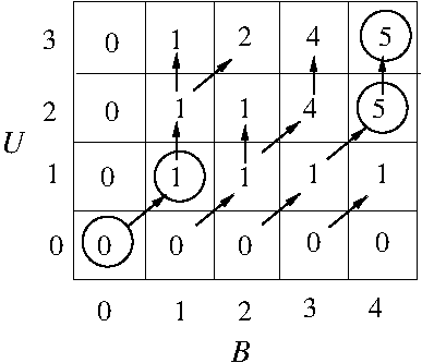
  • Example: Versions of the Knapsack problem that allow greedy and dynamic programming / combinatorial solution-space tree algorithms (pages 425-427).
    • Consider the knapsack instance U = {u1, u2,u3) with B = 50 such that s(u1) = 10, s(u2) = 20, s(u3) = 30, v(u1) = 60, v(u2) = 100, and v(u3) = 120.
    • The optimal 0/1 knapsack load is {u2,u3} with value v(u2) + v(u3) = 100 + 120 = 220. No optimal solution can include u1, which would be greedily selected by greatest value per size-unit. Indeed, optimal solutions for 0/1 Knapsack must be computed by DP or CST algorithms.
    • The optimal fractional knapsack load is all of u1, all of u2, and 2/3 of u3, which has value (1.0 * v(u1) + (1.0 * v(u2) + (2/3 *v(u3) = 60 + 100 + 80 = 240. Indeed, optimal solutions for Fractional Knapsack can be easily computed by a trivial greedy algorithm.
  • Potential exam questions

Thursday, February 20

• In-class exam #1.

Tuesday, February 25

• Midterm break; no lecture..

Thursday, February 27

• Midterm break; no lecture..

Tuesday, March 4 (Lecture #11)
[Sections 22.1-2]

• Went over In-Class Exam #1.
• Exploiting Data Structures
  • The techniques we've seen so far use properties of solution spaces to organize efficient searches of these spaces; in many cases, we have lowered time complexities from exponential to low-order polynomial.
  • A trivial lower bound on the time complexity of many algorithms is a linear function of the given input size as one must read the complete problem input, cf. binary search. To get as close as possible to this bound, need to choose data structures that provide best time complexities for operations required by an algorithm.
  • Example: Exploiting data structures to solve the Minimum Spanning Tree problem
    • Kruskal's algorithm
      • Running time
        = O(|V|(T(MAKE-SET)) + 2|E|(T(FIND-SET)) + |E|(T(UNION)) + SORT(|E|))
        = O(|V|(T(MAKE-SET)) + |E|(T(FIND-SET)) + |E|(T(UNION)) + O(|E| log |E|))
        = O(|V|(T(MAKE-SET)) + |E|(T(FIND-SET)) + |E|(T(UNION)) + O(|E| log |V|^2))
        = O(|V|(T(MAKE-SET)) + |E|(T(FIND-SET)) + |E|(T(UNION)) + O(|E| log |V|))
        
      • Running time relative to various data structures for disjoint sets (see here for more details about cited data structures):

        Data Structure	Time Complexity (Worst Case)
        	MAKE-SET	FIND-SET	UNION	Kruskal's Algorithm
        List (naive)	O(1)	O(n)	O(1)	O(|E||V|)
        List (rep-ptr)	O(1)	O(1)	O(n)	O(|E||V|)
        Forest (naive)	O(1)	O(n)	O(1)	O(|E||V|)
        Forest (rep-ptr)	O(1)	O(1)	O(n)	O(|E||V|)
        Forest (UR + PC)	O(1)	O(1)	O(1)	O(|E| log |V|)

        Note that the O(1) runtimes of Kruskal's algorithm relative to the forest implementation of the disjoint sets abstract data type under the Union-by-Rank (UR) and path-compression (PC) heuristics are actually averages over sequences of operations and requires somewhat intricate proofs of correctness (Section 21.4).

    • Prim's algorithm
      • Running time = O(T(BUILD) + |V|T(EXTRACT-MIN)) + |E|(T(DECREASE-KEY)))
      • Running time relative to various data structures for priority queues (see here for more details about cited data structures):

        Data Structure	Time Complexity (Worst Case)
        	BUILD	EXTRACT- MIN	DECREASE- KEY	Prim's Algorithm
        Array (Unsorted)	O(n)	O(n)	O(n)	O(|E||V|)
        Linked list (Unsorted)	O(n)	O(n)	O(n)	O(|E||V|)
        Array (Sorted)	O(n log n)	O(n)	O(n)	O(|E||V|)
        Linked list (Sorted)	O(n log n)	O(1)	O(n)	O(|E||V|)
        Search tree	O(n)	O(n)	O(n)	O(|E||V|)
        Balanced search tree	O(n)	O(log n)	O(log n)	O(|E| log |V|)
        Binary heap	O(n)	O(log n)	O(log n)	O(|E| log |V|)

  • There are several lessons encoded in the tables above:
    • To obtain the best overall set of running times for a set of operations relative to an abstract data type, a complex underlying data structure may be required.
    • When one is dealing with an algorithm that only invokes a subset of the operations relative to an abstract data type, the best overall data structure implementing that data type may not be appropriate -- rather, one looks for a data structure that gives the best running times for the required subset of operations.
• An efficient algorithm is a collaboration between an appropriate algorithm design technique and one or more data structures whose operation-sets are optimally efficient for the subset of operations required by the algorithm. Hence, need good knowledge of both algorithm design techniques and data structures to create efficient algorithms.
• An algorithm designer also needs a good knowledge of the best-known algorithms for standard problems. After all, who wants to reinvent the wheel?
• Such knowledge tends to be domain-specific. Let's concentrate on the domain of graphs and standard graph algorithms.
• Graph algorithms
  • Why use graphs?
    • Graphs are the natural way to represent any situation in which there are entities and relationships between entities.
  • Representations of graphs (Section 22.1)
    • Two basic choices:
      • Adjacency list
      • Adjacency matrix
    • Adjacency list more compact for sparse graphs, i.e., graphs such that |E| << |V|(|V| - 1)/2; however, as they store only one bit per adjacency, adjacency matrices better for non-sparse graphs.
    • Common operations on graphs:
      • next-adj(v): Return next vertex in enumeration of vertices adjacent to v.
      • adj(v, v'): Return TRUE if v is adjacent to v' in G and FALSE otherwise.
    • Representations differ in terms of the efficiency of these operations.

      Data Structure	Time Complexity (Worst Case)
      	NEXT-ADJ	ADJ
      Adjacency List	O(1)	O(|V|)
      Adjacency Matrix	O(|V|)	O(1)

    • As with any data structure, need to optimize graph representation to algorithm in terms of number of type of operations used.
  • Graph traversal
    • Graph traversal useful in two ways:
      • Visit all nodes in a graph.
      • Impose annotation / structure on the vertices and/or edges of a graph that has subsequent uses.
    • Two types of graph traversal: breadth-first search (BFS) and depth-first search (DFS); let us focus on the former.
    • Breadth-first search on general graphs (Section 22.2)
      • Intuition: Exploration of shells of vertices at successively larger distances from a selected point.
      • ALGORITHM: Basic BFS "chasis"

         1.  BFSBasic(G, s)
         2.     for each vertex u in G - {s} do
         3.        color[u] = white
         4.     color[s] = gray
         5.     Q = {}
         6.     ENQUEUE(Q, s)
         7.     while Q is not empty do
         8.        u = DEQUEUE(Q)
         9.        for each v in adj[u] do
        10.           if color[v] = white then
        11.              color[v] = gray
        12.              ENQUEUE(Q,v)
        13.        color[u] = black
        

      • Interpretation of colors:
        • black = fully explored (node + children)
        • gray = partially explored (node only)
        • white = unexplored
        • Visualize as ink spreading from a central point outwards along edges until it has reached all vertices in a graph.
      • Analysis of running time
        • Running time = |V|O(1) + |Q|O(1) + |E|O(1) + T_tot(next-adj)) = |V| + |V|O(1) + |E| + T_tot(next-adj)) = O(|V| + |E| + T_tot(next-adj))
          • Adjacency list: O(|V| + |E| + |E|) = O(|V| + |E|) time
          • Adjacency matrix: O(|V| + |E| + |V|^2) = O(|V|^2) time
        • Though |E| <= |V|(|V| - 1)/2 = O(|V|^2), often keep |E|-term in expressions to show running time relative to sparse graphs.
        • Did not analyze algorithm in terms of rigorously-derived T(n) function -- worked less formally and directly in terms of big-Oh behavior of individual algorithm components.
        • Did not analyze algorithm by nested control structure -- had to reason about behavior of algorithm as a whole to derive certain quantities, e.g., total length of queue over execution of algorithm.

Tuesday, March 4

• In-class Exam #2 Notes
  I've finished making up the second in-class exam. The exam will be closed-book and written in-class on paper (please bring your own pens). It will be 75 minutes long and has a total of 50 marks (this is not coincidental; I have tried to make the number of marks for a question approximately equal to the number of minutes it should take you to do it in the best case). The exam will cover material in course lectures #5 through #12 inclusive (Topics 4-6 in the potential exam question list). There will be three questions:
  1. Greedy / Graph Algorithms [Topics 5 and 6] (2 parts / 20 marks)
  2. D&C / Dynamic Programming / Greedy Algorithms [Topics 4 and 5] (2 parts / 20 marks)
  3. D&C / Dynamic Programming Algorithms [Topic 4] (2 parts / 10 marks)

  I hope the above helps, and I wish you all the best of luck with this exam.

Thursday, March 6 (Lecture #12)
[Sections 22.2 and 24.1]

• Graph algorithms (Cont'd)
  • Graph traversal (Cont'd)
    • ALGORITHM: Full BFS (page 595)

       1.  BFSFull(G, s)
       2.     for each vertex u in G - {s} do
       3.        color[u] = white
       4. **     d[u] = INFTY
       5. **     pi[u] = nil
       6.     color[s] = gray
       7. **  d[s] = 0
       8.     Q = {}
       9.     ENQUEUE(Q, s)
      10.     while Q is not empty do
      11.        u = DEQUEUE(Q)
      12.        for each v in adj[u] do
      13.           if color[v] = white then
      14.              color[v] = gray
      15. **           d[v] = d[u] + 1
      16. **           pi[v] = u
      17.              ENQUEUE(Q,v)
      18.        color[u] = black
      

      Starred (**) lines are those added relative to basic BFS algorithm given previously.
    • What are the pi and d arrays for?
      • BFS defines a search tree based on all vertices of G that is rooted at the start vertex s; the pi-array defines the node-parent relations in this tree.
      • This search tree is structured such that the length of the path from s to u in this tree is the length of the shortest path (in terms of # edges) between s and u in G; the d-array contains these shortest-path length values.
      • Intuition behind proof of correctness for d-values: If there were a shorter path from s to v via some vertex u, during exploration of children of u, v would have previously been colored gray!
      • Can use BFS to derive shortest paths (in terms of # edges on path) between a specified vertex s and all other vertices in a graph.
    • Example: Sample run of BFS algorithm (page 596). [Diagram]
      • Courtesy of the expanding-shell nature of BFS, shortest paths once found are never revised, cf., Dijkstra's algorithm (see below).
    • Note that Prim's algorithm for computing minimum spanning trees is somewhat like BFS; both are expanding a frontier outwards from an initial vertex in the graph, but while BFS expands this frontier uniformly by distance from the start point, the expansion by Prim is relative the the smallest-weight edge extending into the frontier (this is done by replacing an ordinary queue with an appropriately-keyed priority queue).
  • Shortest Paths in Edge-Weighted Graphs
    • Assume edge-weights are specified in a matrix w(), i.e., w(u,v) is the weight of the edge between vertices u and v in a given graph (= +INFINITY if there is no such edge). Note that negative edge-weights are possible.
    • Has many applications depending on how you interpret the edge-weights, e.g., distances, costs.
    • Can solve by applying edge-expansion and ordinary BFS; however, this yields an exponential time algorithm. Can we do better?
    • Two types of problems:
      • Single-source shortest paths
      • All-pairs shortest paths
    • Can further break down algorithms based on whether or not they detect negative-weight cycles. Such cycles are problematic because they render shortest-paths estimates meaningless, e.g., can make length of path arbitrarily short by appropriate number of traversals around the cycle.
    • Example: A graph with a negative-weight cycle.

      

      Observe that in this graph, a shortest path from A to C can always be made shorter by including one more time around the negative-weight cycle B->D->B.
    • Properties of shortest paths:
      • Triangle inequality: d(s,v) <= d(s,u) + w(u,v)
      • Shortest path has at most |V| - 1 edges, i.e., can eliminate negative-, zero-, and positive-weight cycles from shortest paths.
      • Shortest paths satisfy the optimal substructure property, i.e., given a shortest path from s to v and a vertex u on this path, the subpaths s->u and u->v are also shortest paths; this means that there are many nice algorithmic possibilities, i.e., DP, D&C, Greedy.
    • The Relax operation
      • ALGORITHM: Relax (pages 648-649)

         1.  InitSingleSource(G, s)
         2.     for each vertex v in adj[v] do
         3.        d[v] = INFTY
         4.        pi[v] = nil
         5.     d[s] = 0
        
         6.  Relax(u, v, w)
         7.     if (d[v] > d[u] + w(u,v)) then
         8.        d[v] = d[u] + w(u,v)
         9.  	   pi[v] = u
        

      • Example: Two sample applications of the Relax operation.

        

      • The relax operation is trivial; however, sequences of relaxations can be quite powerful.
      • All algorithms we consider for shortest path problems will essentially differ only in the the order in which edges are relaxed and the number of times each edge is relaxed.

Tuesday, March 11 (Lecture #13)
[Section 24.3]

• Graph Algorithms (Cont'd)
  • Single-source shortest paths algorithms
    • Dijkstra's algorithm (Section 24.3)
      • This algorithm essentially applies relaxations in a systematic matter to grow a set of vertices with known shortest-path distances outwards from the source vertex to encompass the whole graph. In particular, relaxations are applied to vertices (or rather, the adjacencies of those vertices) as they are added to this set and can be seen as extending out from the frontier of this region into the remainder of the graph.
      • ALGORITHM: Dijkstra (page 658)

         1.  Dijkstra(G, w, s)
         2.     Initialize-Single-Source(G, s)
         3.     S = {}
         4.     Q = V[G]
         5.     while Q is not empty do
         6.        u = EXTRACT-MIN(Q)
         7.        S = S u {u}
         8.        for each vertex v in adj[u] do
         9.           Relax(u, v, w)
        

      • Example: Sample run of Dijkstra's algorithm (no negative weight cycle).

        

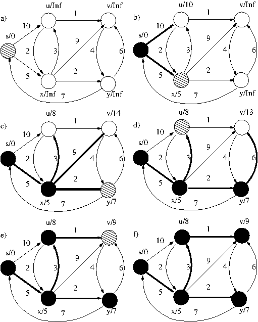
        Part (a) shows the initial state of the graph and subsequent parts show the graph after a particular vertice's adjacencies have been relaxed. Black vertices are fully relax-processed and the shaded vertex is the vertex whose adjacencies will be relaxed in the next part. d-values are written next to vertex names and pi-values are implicit in the thick edges.

      • Note that Dijkstra's algorithm, unlike BFS, can change the shortest path tree rooted at the start vertex over an algorithm execution -- this is because newly-encountered weighted edges can revise previously-found shortest paths.
      • Example: Sample run of Dijkstra's algorithm (page 659). [Diagram]
      • Analysis of running time
        • Running time
          = T(INITIALIZE) + |V|T(EXTRACT-MIN) + |E|T(RELAX)
          = T(INITIALIZE) + |V|T(EXTRACT-MIN) + |E|T(DECREASE-KEY)
          
        • Runs in O(|E| log |V|) time relative to a binary heap.
      • Doesn't Dijkstra's algorithm look an awful lot like Prim's algorithm for minimum spanning trees? It should! Try writing the code for the initialization and relaxation procedures into Dijkstra's algorithm, eliminating the S-lines (which are not being used), and then comparing with Prim's algorithm -- oddly enough, you'll see that relaxation is a generalization of the key-value adjustment done by Prim on lines 11 and 12, e.g.,

         1.  DijkstraRewrite(G, w, s)
         2.     for each u in V do
         3.        d[u] = INFTY
         4.        pi[u] = nil
         5.     d[s] = 0
         6.     Q = V
         7.     while Q not empty do
         8.        u = EXTRACT-MIN(Q)
         9.        for each v in adj[u] do
        10.           if d[u] + w(u,v) < d[v] then
        11.              d[v] = d[u] + w(u, v)
        12.              pi[v] = u
        

      • Dijkstra's algorithm cannot detect negative cycles, and will produce erroneous results if one or more such cycles are present. Worse, this algorithm may fail in the presence of negative-weight edges, independent of whether these edges are part of a negative-weight cycle.
      • Example: Sample run of Dijkstra's algorithm (negative weight cycle).

        

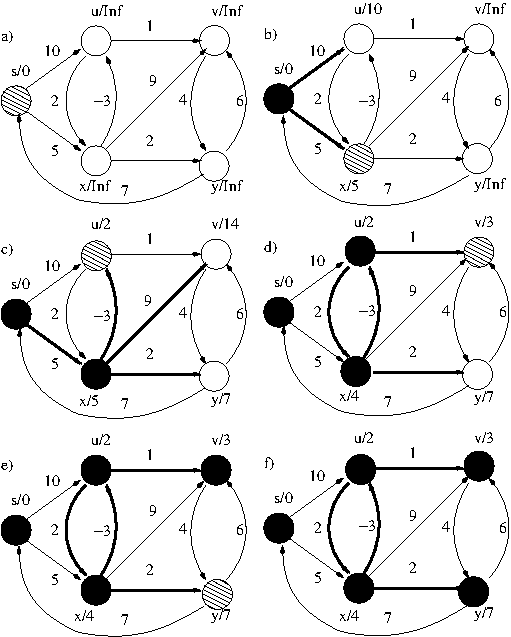
    • Dijkstra's algorithm is fast, but at the price of restricted applicability. Can we do better?
    • The Bellman-Ford algorithm (Section 24.1)
      • This algorithm essentially adopts the philosophy that if you invoke relaxation often enough, all will be well. Oddly enough, it turns out that if you relax each edge in the graph |V| - 1 times, the d-values associated with all vertices are guaranteed to settle to the actual shortest-distance values. This works because each round of relaxations relaxes one edge further along a shortest path and each shortest path has at most |V| - 1 edges.
      • ALGORITHM: `Bellman-Ford (page 651)

         1.  BellmanFord(G, w, s)
         2.     Initialize-Single-Source(G,s)
         3.     for i = 1 to |V| - 1 do
         4.        for each edge (u,v) in E do
         5.           Relax(u, v, w)
         6.     for each edge (u,v) in E do
         7.        if d[v] > d[u] + w(u,v) then
         8.           return FALSE
         9.    return(TRUE)
        

      • Example: Sample run of Bellman-Ford algorithm (no negative weight cycle).

        

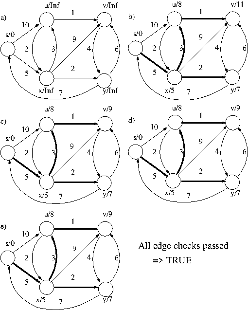
        Edges are relaxed in the following order in each relaxation-phase: (s,u). (s,x), (u,v), (u,x), (u,y), (v,y), (x,u), (x,y), (y,s), (y,v). d-values are written next to vertex names and pi-values are implicit in the thick edges.

      • Example: Sample run of the Bellman-Ford algorithm (page 652). [Diagram]
      • Running time = O(|V||E|)
      • This algorithm does (|V| - 1)|E| relaxations, as compared to the |E| relaxations done by Dijkstra's algorithm, and hence runs much slower. However, it has the advantage of being able to detect negative-weight cycles.
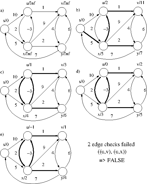
        • The intuition behind this is almost the same as for the Bellman-Ford algorithm in general as given above -- in addition to propagating correct shortest distances along a path, the invoked relaxations propagate the negative summed weights around negative-weight cycles and dump these negative weights onto regular paths, where the resulting screwup in the relation between d-values of adjacent vertices can be detected by a simple scan of all edges (lines 7-9 of the algorithm)
        • Shouldn't Dijkstra's algorithm be able to detect negative-weight cycles by the same argument? I suspect not, as Dijkstra's algorithm probably does not invoke enough relaxations to guarantee that the influences of negative-weight cycles will necessarily be dumped onto all (or even any) paths -- however, I could be wrong in this.
      • Example: Sample run of Bellman-Ford algorithm (negative weight cycle).

        

    • Note that the running times given for both Dijkstra's algorithm and the Bellman-Ford algorithm assume that the input graph is represented as an adjacency list -- if the graph is instead represented as an adjacency matrix, the running time of both algorithms becomes O(|V|^3).

Thursday, March 13

• In-class exam #2.

Tuesday, March 18 (Lecture #14)
[Sections 25.1-2; Class Notes]

• Went over answers to in-class exam #2.
• Graph algorithms (Cont'd)
  • All-pairs shortest paths algorithms (Section 25)
    • Can do this by applying either of the algorithms for single-source shortest paths |V| times (once for each vertex in the graph). Is there a faster way? Try dynamic programming!
      • Note that constructing the actual shortest paths in all-pairs shortest paths is more complex than for single-source shortest paths and will not be covered here.
    • Unlike our previous shortest-path algorithms, our all-pairs shortest-paths algorithms will use a matrix W that is a fusion of the adjacency matrix and edge-weight function defined as follows:

      Wi,j= {	0	if i == j
      	w(i,j)	if i <> j and (i,j) in E
      	INFTY	if i <> j and (i,j) not in E

    • Some recurrences for shortest paths
      • Path-length based

        L(0)i,j= {	0	i == j
        	INFTY	i <> j

        L(m)i,j = min1 <= k <= |V|{

        L(m-1)i,k + Wk,j

        }

        where L^(m)_i,j, 0 <= m <= |V| - 1, is the length of the shortest path in G between vertices vi and vj with at most m edges.
      • Intermediate-vertex-set based:

        D⁽⁰⁾_i,j = W_i,j
        D^(m)_i,j = min { D ^(m-1)_i,j ,     D ^(m-1)_i,m + D ^(m-1)_m,j}

        where D⁽⁰⁾_i,j is the length of the shortest path in G between vi and vj with no intermediate vertices and D^(m)_i,j, 1 <= m <= |V|, is the length of the shortest path in G between vertices vi and vj with intermediate vertices in the set {v1, v2, ..., vm}.
    • These algorithms will now be creating matrices instead of vectors of shortest-path distances; moreover, they will operate on adjacency matrix representations of input graphs instead of adjacency lists.
    • Shortest paths and matrix multiplication (Section 25.1)
      • Uses first (path-length based) recurrence above.
      • ALGORITHM: Extending Shortest Paths subroutine

         1.  ExtendShortestPaths(L, W)
         2.     n = rows[L]
         3.     Create n x n matrix L'
         4.     for i = 1 to n do
         5.         for j = 1 to n do
         6.             L'_ij = INFTY
         7.             for k = 1 to n do
         8.                 L'_ij = min(L'_ij, L_ik + W_kj)
         9.     return L'
        

      • Yes, this does look a lot like matrix multiplication. Odd, isn't it? There are some deep mathematical reasons for this, tied up with a mathematical structure common to both problems that is called a closed semiring (the interested are referred to Section 27.5 in the first edition of the textbook for more details).
      • ALGORITHM: All Pairs Shortest Paths (slow version; runs in (O(|V|^4) time)

         1.  AllPairsShortestPathsSlow(W)
         2.     n = rows[W]
         3.     L^(1) = W
         4.     for m = 2 to n - 1 do
         5.         L^(m) = ExtendShortestPaths(L^(m - 1), W)
         6.     return L^(n - 1)
        

      • Example: Sample run of the slow algorithm (page 690).
      • Why grow paths slowly one edge at a time? If we send L^(m - 1) twice to EXTEND-SHORTEST-PATHS instead of L^(m - 1) and W, the path-length will increase at an exponential rate and be >= |V| - 1 in only log |V| calls to ExtendShortestPaths!
      • ALGORITHM: All Pairs Shortest Paths (fast version; runs in O(|V|^3 log |V|) time)

         1.  AllPairsShortestPathsFast(W)
         2.     n = rows[W]
         3.     L^(1) = W
         4.     m = 1
         5.     while m < n - 1 do
         6.        L^(2 * m) = EXTEND-SHORTEST-PATHS(L^(m), L^(m))
         7.  	   m = 2 * m
         8.     return L^(m)
        

    • The Floyd-Warshall algorithm (Section 25.2)
      • Uses second (intermediate-vertex-set based) recurrence above.
      • ALGORITHM: Floyd-Warshall

         1.  APSPFloydWarshall(W)
         2.     n = rows[W]
         3.     D^(0) = W
         4.     for k = 1 to n do
         5.         Let D^(k) be a new n x n matrix
         6.         for i = 1 to n do
         7.             for j = 1 to n do
         8.                 D^(k)_ij = min(D^(k - 1)_ij, 
         9.                                D^(k - 1)_ik + 
        10.                                D^(k - 1)_kj)
        11.     return D^(n)
        

      • Example: Sample run of the Floyd-Warshall algorithm (page 690).
      • Running time = O(|V|^3)
    • Note that both of these algorithms are technically operating on a 3-D matrix of size O(|V|^3); however, as we only need to save adjacent 2-D "slices" of this matrix, we actually use O(|V|^2) space.
    • Note that the running times given for the three algorithms above assume that the input graph is represented as an adjacency matrix -- if the graph is instead represented as an adjacency list, the running times of each algorithm increase by a a multiplicative factor of |V|!
  • INTERLUDE: A look at the mechanics of Assignment #3.
• Potential exam questions
• Using the techniques we've talked about so far in this course, we can often derive a polynomial-time algorithm for a problem of interest and hence prove that this problem is solvable in polynomial time, i.e., the problem is (polynomial-time) tractable.
• However, suppose we run across a problem for which we cannot find a polynomial time algorithm, e.g., 0/1 Knapsack. Are we just not thinking hard enough or is it really the case that there isn't a polynomial-time algorithm for that problem, i.e., the problem is (polynomial-time) intractable?
• Proving Polynomial-Time Intractability
  • Two types of proofs:
    • Absolute (based on examining the problem in isolation)
      • Lower bound theory / information-theoretic arguments.
    • Relative (based on examining a problem in relation to other problems)
      • Based on the concept of a reduction, where a reduction between problems A and B is essentially an algorithm that solves instances of A by calling a subroutine for solving instances of B.
  • Example: A reduction from problem A to problem B.

    

  • Let's focus on the relative approach, in particular, polynomial-time reductions, i.e., reductions whose associated transformations run in polynomial time and make a polynomial calls to the subroutine for B, where the polynomials are in terms of the input size for A.
  • Three very useful properties of polynomial-time reductions:
    1. Polynomial-time solvability passes backwards along a reduction, i.e., if A reduces to B and B is solvable in polynomial time than A is solvable in polynomial time.
    2. Polynomial-time unsolvability passes forwards along a reduction, i.e., if A reduces to B and A is not solvable in polynomial time than B is not solvable in polynomial time.
    3. Polynomial-time reductions are transitive, i.e., if A reduces to B and B reduces to C then A reduces to C.

            Polynomial-time solvability
    
    	      <-------------
            A reduces to B reduces to C
    	      ------------->
    
           Polynomial-time unsolvability
    

Thursday, March 20 (Lecture #15)
[Sections 34.1-34.2; Class Notes]

• Proving Polynomial-Time Intractability (Cont'd)
  • Example: Fun with Reduction Webs I: Supose we have a set of problems {A, B, C, D, E, F, G, H} with the following reductions between them:
    • A polynomial-time reduction from A to B
    • A polynomial-time reduction from A to C
    • An exponential-time reduction from B to D
    • A polynomial-time reduction from C to E
    • A polynomial-time reduction from D to F
    • A polynomial-time reduction from E to B
    • A polynomial-time reduction from E to G
    • An exponential-time reduction from E to H
    What do we know about the polynomial-time (un)solvability of our problems relative to each of the following:
    1. A is polynomial-time unsolvable
    2. E is polynomial-time solvable
    3. F is polynomial-time solvable
    4. C is polynomial-time unsolvable
    5. H is polynomial-time unsolvable
    6. A is polynomial-time solvable
    7. G is polynomial-time unsolvable
  • The upshot is, all we need is one polynomial-time intractable problem to get the ball rolling! But where do we find such a problem?
  • Our quest for a "seed" polynomial-time intractable problem will have two phases:
    1. Demonstrating that we need only focus on decision problems.
    2. Isolating polynomial-time intractable decision problems.
  • Can use reductions to show that we only need to concern ourselves with decision versions of problem -- can usually show that polynomial-time solvability and unsolvability propagates to cost and example versions.
  • Example: Some computational problems that we will be looking out (handout) [PDF]

    Vertex Cover (VC)
    Input: An undirected graph G = (V,E) and an integer k > 0.
    Question: Is there a vertex cover of G of size at most k, i.e, is there a subset V' \subseteq V such that |V'| <= k and for all edges (u,v) \in E, at least one of u and v is in V'?

    Vertex Cover Cost (VC-C)
    Input: An undirected graph G = (V,E).
    Output:} The size of the smallest vertex cover of G.

    Vertex Cover Example (VC-E)
    Input: An undirected graph G = (V,E).
    Output: One of the smallest vertex covers of G.

    Clique
    Input: An undirected graph G = (V,E) and an integer k > 0.
    Question: Is there a clique in G of size at least k, i.e., is there a subset V' \subseteq V, |V'| >= k, such that for all u, v \in V', (u,v) \in E?

    Subset sum (SS)
    Input: A set S of integers and an integer k \geq 0.
    Question: Is there a subset S' of S whose elements sum to k?

    Steiner tree in graphs (STG)
    Input: An undirected graph G = (V,E), a set V' \subseteq V, and an integer k > 0.
    Question: Is there a tree in G that connects all vertices in V' and contains at most k edges?

  • Example Reductions between different vertex cover problems.
    • Vertex Cover (Decision) is solvable in polynomial time if and only if Vertex Cover (Cost) is solvable in polynomial time.
      • if Vertex Cover (Cost) is solvable in polynomial time then Vertex Cover (Decision) is solvable in polynomial time: Prove by giving a polynomial time reduction from Vertex Cover (Decision) to Vertex Cover (Cost):

        VERTEX-COVER-DECISION(G, k)
            if (VERTEX-COVER-COST(G) <= k) then
                return(TRUE)
            else
                return(FALSE)
        

      • If Vertex Cover (Decision) is solvable in polynomial time then Vertex Cover (Cost) is solvable in polynomial time: Prove by giving a polynomial time reduction from Vertex Cover (Cost) to Vertex Cover (Decision):

        VERTEX-COVER-COST(G)
            k = 1
            while not VERTEX-COVER-DECISION(G,k) do
                k = k + 1
            return(k)
        

    • Vertex Cover (Decision) is solvable in polynomial time if and only if Vertex Cover (Example) is solvable in polynomial time.
      • if Vertex Cover (Example) is solvable in polynomial time then Vertex Cover (Decision) is solvable in polynomial time: Prove by giving a polynomial time reduction from Vertex Cover (Decision) to Vertex Cover (Example):

        VERTEX-COVER-DECISION(G, k)
            if (cost(VERTEX-COVER-EXAMPLE(G))) <= k then
                return(TRUE)
            else
                return(FALSE)
        

      • If Vertex Cover (Decision) is solvable in polynomial time then Vertex Cover (Example) is solvable in polynomial time: Prove by giving a polynomial time reduction from Vertex Cover (Example) to Vertex Cover (Decision):

        VERTEX-COVER-EXAMPLE(G)
        
            min_cost = 1
            while not VERTEX-COVER-DECISION(G,min_cost) do
                min_cost = min_cost + 1
        
            k = min_cost
            S = {}
            G' = G
            while |S| < min_cost do
                for each vertex v' in V' do
                    G'' = (V' u {x}, E' u {(v',x)})
                    if (VERTEX-COVER-DECISION(G'',k)) then
                        S = S u {v'}
                        G' = G' - {v'}
                        k = k - 1
                        break
            return(S)
        

        • Reduction uses vertex x and edge attached to x as ``probe'' to see if vertex v' is in the vertex cover. If it is, edge (v',x) is covered by the current cover (VERTEX-COVER-DECISION(G'',k) = TRUE); otherwise, x must be added to cover, creating a cover of size k + 1, rendering VERTEX-COVER-DECISION(G'',k) = FALSE.
  • Focusing on decision problems makes our lives much easier when dealing with reductions. Indeed, we can make things even simpler by using just one type of reduction.
    • A (polynomial time) many-one reduces to B if there is a polynomial-time function f() that transforms instances of A into instances of B such that the answer to instance I of A is "yes" if and only if the answer to instance f(I) of B is "yes".
  • Example: A many-one reduction from decision problem A to decision problem B.

    

Tuesday, March 25 (Lecture #16)
[Sections 34.3-34.5; Class Notes]

• Proving Polynomial-Time Unsolvability (Cont'd)
  • Example: Clique many-one reduces to Vertex Cover (Lemma 3.1, Garey and Johnson (1979))
    • Relies on a nice graph-theoretic characterization of cliques and vertex covers on the same set of vertices.
    • Define the complement Gc = (V,Ec) of a graph G = (V,E) as the graph on V with edge-set Ec = {(u,v) | (u,v) is not in E}.
    • Given an instance (G,k) of CLIQUE, the reduction constructs an instance (Gc,|V| - k) of VC.
    • Prove that the given instance of CLIQUE has answer "yes" iff the constructed instance of VC has answer "yes":
      • If the given instance of CLIQUE has answer "yes" then the constructed instance of VC has answer "yes": Consider a solution S \subseteq V of size k to the given instance of CLIQUE. As each pair of vertices in S is connected by an edge in G, no pair of vertices in S is connected by an edge in Gc. Hence, V - S is a vertex cover of size |V| - k in the constructed instance of VC.
      • If the constructed instance of VC has answer "yes" then the given instance of CLIQUE has answer "yes": Consider a solution S \subseteq V of size |V| - k in Gc to the constructed instance of VC. Consider S' = V - S. None of the vertices in S' are connected by an edge in Gc (else, one of them would have to be in the vertex cover). Hence, there is an edge between each pair of vertices in S' in G, and S' is a clique of size k in the given instasnce of CLIQUE.
  • Example: Subset Sum many-one reduces to 0/1 Knapsack
    • Need decision version of 0/1 Knapsack:

      0/1 Knapsack (decision version) (01KN)
      Input: A set U of items, an item-size function s(), an item-value function v(), and positive integer B and k.
      Question: Is there a subsets U' of U such that the sum of the sizes of the items in U' is less than or equal to B and the sum of the values of the items in U' is at least k?

    • Given an instance (S = {s1,..,sn},t) of SS, construct an instance (U,s,v,B,k) of 01KN such that U = {u1,..,un} where s(ui) = v(ui) = si, 1 <= i <= n, and B = k = t.
    • Prove that the given instance of SS has answer "yes" iff the constructed instance of 01KN has answer "yes":
      • If the given instance of SS has answer "yes" then the constructed instance of 01KN has answer "yes": Consider a solution S' = {s'1,..,s'm} \subseteq S for the given instance of SS. Construct a candidate solution U' for the constructed instance of 01KN consisting of the items corresponding to the selected numbers in S'. Observe that the summed size and value of this solution is t = B = k, meaning that U' is a solution.
      • If the constructed instance of 01KN has answer "yes" then the given instance of SS has answer "yes": Consider a solution U' to the constructed instance of 01KN. As item values and sizes are the same, the solution size and value most be the same. Thus, if the summed size is <= B and the summed value is >= k, the summed size must be B = k = t. Thus, one can easily construct a solution for the given instance of SS consisting of those integers in S corresponding to items in U'.
  • Example: Vertex Cover many-one reduces to Steiner Tree in Graphs (Day, Johnson, and Sankoff (1986))
    • Given and instance (G = (V,E),k) of VC construct an instance (G' = (V',E'),V'',k') of STG such that V' = {r} u {v'1,..,v'|V|} u {e'1,..,e'|E|}, E' = {(r,v'i) | 1 <= i <= |V|} u {(v'i,e'j) | vertex i is an endpoint of edge j in E}, V'' = {r} u {e'1,..,e'|E|}, and k' = k + |E|.
    • This reduction requires that solutions to the constructed instance of STG have a three-level structure in which the top level is the root-vertex r, the second level consists of vertices corresponding to the edges in G, and the vertices in the second level correspond to vertices in a vertex cover for G.
    • Prove that the given instance of VC has answer "yes" iff the constructed instance of STG has answer "yes":
      • If the given instance of VC has answer "yes" then the constructed instance of STG has answer "yes": Consider a solution S \subseteq V of size k for the given instance of VC. For each edge e in E, let end(e) be the endpoint of e in S (if they are both in S, pick one arbitrarily). The tree in G' consisting of V' and the vertices v'i corresponding to vertices in S, along with the edges linking these vertices to r and the vertices e'j (that is, for each vertex e'j corresponding to edge j in E, select edge (e'j,end(j))), is a solution for the constructed instance of STG that contains k + |E| edges.
      • If the constructed instance of STG has answer "yes" then the given instance of VC has answer "yes": A solution tree for the constructed instance of STG of size k' must have at least one edge from r ro some v'i, but may have multiple pairs of edges that form "wedges" ((v'i,e'j),(v'k,e'j) where there is an edge (r,v'i) in the tree but no edge (r,v'k)). Note that each wedge can be replaced by the edge-pair ((r,v'k),(v'k,e'j)) without changing the cost of the tree. The tree resulting after all such replacements are made will have k edges from r to various v'i and |E+| edges from various v'i to various e'j. The vertices v'i correspond to vertices in G that form a vertex cover of size k.
  • Now we have to isolate a polynomial-time intractable decision problem ... Oddly enough, reductions can help us further in this, if used in tandem with problem classes.
  • A problem class is a set of problems that has a particular type of algorithm.
  • Example: Class P is the set of all decision problems that have polynomial-time algorithms.
  • Use reductions to isolate the most computationally difficult problems in a problem class C using the notions of problem hardness and completeness.
    • A problem A is C-hard if every problem in C reduces to A -- if A is also in C, it is C-complete.
    • C-hard problems are as hard as the hardest problems in C.
    • C-complete problems are the hardest problems in C.
  • Need a class C of decision problems that properly includes (or is widely believed to properly include) class P and for which we have hard / complete problems -- can then use these C-hard / -complete problems as basis for reductions to show that problems of interest to us are not in P and hence are not solvable in polynomial time.
    

  • Example: Class EXPTIME is the set of all decision problems that have exponential-time algorithms.
  • Decision versions of all problems we've looked at so far are in EXPTIME.
  • Example: VERTEX COVER is in EXPTIME courtesy of the algorithm that in O(2^{|V|}) time generates all subsets of vertices in the given graph and then for each such candidate vertex cover V' verifies in O(|E||V'|) time that every edge in G has an endpoint in V'.
  • Example: KNAPSACK is in EXPTIME courtesy of the algorithm that in O(2^{|U|}) time generates all subsets of item-set U and then for each such candidate knapsack-load U' verifies in O(|U'|) time that the summed size of the items in U' is <= B and the summed value of the items in U' is >= k.
  • Example: STEINER TREE IN GRAPHS is in EXPTIME courtesy of the algorithm that in O(2^{|E|}) time generates all subsets of edge-set E and for each such candidate edge-set E' verifies in polynomial time that there are <= k edges in E' and these edges form a tree in G that connects all vertices in V'.
  • Example: Class NP is the set of all decision problems that have nondeterministic polynomial-time algorithms, i.e., problems such that candidate solutions can be verified in polynomial time.
  • Decision versions of all problems we've looked at so far are in NP.
  • Example: VERTEX COVER, KNAPSACK, and STEINER TREE IN GRAPHS are all in NP courtesy of the polynomial time verification algorithms described above.
  • NP is included in EXPTIME, P is included in EXPTIME, and P is included in NP; however. while the first two of these inclusions are proper, it is not known if the third inclusion is proper (hence, the "P = NP?" conjecture). Still, if EXPTIME-complete problems are not useful to us, NP-complete problems might be.
  • Example: Fun with Reduction Webs II: Supose we have a set of problems {A, B, C, D, E, F, G, H} with the following reductions between them:
    • A polynomial-time reduction from A to B
    • A polynomial-time reduction from A to C
    • An exponential-time reduction from B to D
    • A polynomial-time reduction from C to E
    • A polynomial-time reduction from D to F
    • A polynomial-time reduction from E to B
    • A polynomial-time reduction from E to G
    • An exponential-time reduction from E to H
    What do we know about our problems relative to each of the following:
    1. C is in P and E is NP-hard
    2. F is in P and A is NP-complete
    3. E is in P and G is NP-hard
    4. A is in P and F is NP-complete
    5. E is in P and C is NP-hard
  • Now, all we need is one EXPTIME- or NP-hard problem to start the ball rolling ...

Tuesday, March 25

• Final Exam Notes
  I've finished making up the final exam. this exam will be closed-book and written in-class on paper (please bring your own pens). It will be 120 minutes long and has a total of 100 marks (this is not coincidental; I have tried to make the number of marks for a question approximately equal to the number of minutes it should take you to do it in the best case). The exam will cover material in all course lectures. There will be five questions:
  1. Time Complexity (Topic 2) (3 parts / 12 marks)
  2. Algorithm Design Techniques I (Topics 3, 4, and 5) (2 parts / 24 marks)
  3. Graph Algorithms (Topics 5 and 6) (3 parts / 24 marks)
  4. Algorithm Design Techniques II (Topics 3, 4, 5, and 6) (4 parts / 19 marks)
  5. Proving Polynomial Time Unsolvability (Topic 7) (3 parts / 21 marks)

  I hope the above helps, and I wish you all the best of luck with this exam.

Thursday, March 27 (Lecture #17)
[Section 35.1; Class Notes]

• Proving Polynomial-Time Unsolvability (Cont'd)
  • One strategy for obtaining an initial C-hard problem X for class C is to create a generic reduction from any problem in C to X. How might one do this, though?
  • Such a generic reduction is relatively easy to construct for a class C of decision problems relative to a language-recognition machine.
    • Equivalence of decision problems and language acceptance problems (map decision problem to language of bitstrings consisting of instance-encodings of all instances for which answer is "yes").
    • All problems in a class C of decision problems relative to a language-recognition-machine M are reducible to the following problem (which is also typically itself in class C):
      M-Acceptance
      Input: Machine m of type M, input x.
      Question: Does m accept, i.e., produce output "yes", on input x?

  • Example: P is the set of all decision problems whose associated languages of "yes"-instances can be recognized by a polynomial-time deterministic Turing machine (DTM).
  • Example: EXPTIME is the set of all decision problems whose associated languages of "yes"-instances can be recognized by a exponential-time deterministic Turing machine (EDTM).
  • Hence, we have one polynomial-time unsolvable problem -- EDTM-ACCEPTANCE! However, there are many problems of interest for which one cannot construct reductions from EDTM-ACCEPTANCE. Perhaps these problems are not EXPTIME-hard; need something a bit less difficult, computationally-speaking.
  • Example: NP is the set of all decision problems whose associated languages of "yes"-instances can be recognized by a polynomial-time nondeterministic Turing machine (NDTM).
    • Nondeterministic TM may have arbitrary-choice conditional statements; machine computes "yes" on an input if there is some set of choices at these arbitrary-choice conditionals that yields an accepting computation for the given string.
    • Arbitrary-choice conditionals = way of looking at all possible solutions for a given instance within an NDTM! Hence, nicely encodes notion of polynomial-time verification.
    • NDTM ACCEPTANCE is NP-complete!
  • NDTM ACCEPTANCE may appear as unnatural a problem as EDTM ACCEPTANCE at first glance; however, it is not.
  • Two routes to useful NP-complete problems:
    • Historical route
      • NTDM ACCEPTANCE many-one reduces to CNF SATISFIABILITY (Cook (1971))
        • A logic formula is in conjunctive normal form (CNF) if it is the conjunction (AND) of a set of disjunctive (OR) clauses.

          CNF Satisfiability
          Input: A CNF formula F.
          Question: Is there a satisfying assignment for F, i.e., an assignment of values to the variables of F that make F evaluate to True?

        • The reduction is essentially a simulation of an NDTM as a CNF logic formula that describes a sequence of configurations comprising an NDTM computation -- the formula is true iff a sequence of computations leading to string-acceptance exists.
      • CNF SATISFIABILITY many-one reduces to 3-CNF SATISFIABILITY (Karp (1972))
        • A logic formula is in 3-conjunctive normal form (3-CNF) if it is CNF and each clause has exactly three literals.

          3-CNF Satisfiability
          Input: A 3-CNF formula F.
          Question: Is there a satisfying assignment for F?

        • This reduction replaces each CNF clause of strictly less or more than three literals with a set of one or more 3-literal clauses that is true iff the original clause is true.
      • The real genius of Karp (1972) was to show reductions from CNF SATISFIABILITY and 3-CNF SATISFIABILITY to 18 problems of interest drawn from graph theory, scheduling, and network design. This initial list of 18 has since blossomed to several thousand (see the Appendix of Garey and Johnson (1979) for a small but nonetheless significant list of known NP-hard problems).
        • Note that one of Karp's reductions (MINIMUM COVER to STEINER TREE IN GRAPHS) is wrong; however, with a slight modification, the general idea works.
        • Stresses the need for proofs of correctness for reductions.
    • Textbook route
      • NDTM ACCEPTANCE many-one reduces to CIRCUIT SATISFIABILITY (Lemma 34.6)

        Circuit Satisfiability
        Input: A circuit C.
        Question: Is there a set of input-values for C that makes C output true on its output line?

      • CIRCUIT SATISFIABILITY many-one reduces to GENERAL SATISFIABILITY (Theorem 34.9)

        General Satisfiability
        Input: A combinational logic formula F.
        Question: Is there a satisfying assignment for F?

      • GENERAL SATISFIABILITY many-one reduces to 3-CNF SATISFIABILITY (Theorem 34.10)
  • By transitivity of reductions, all problems above are NP-hard. This thus makes for the second (and usually far easier) strategy for proving a problem X C-hard -- that is, give a reduction from known C-hard problem Y to X.
  • Example: 3-CNF SATISFIABILITY many-one reduces to CLIQUE (Theorem 34.11)
  • Example: 3-CNF SATISFIABILITY many-one reduces to SUBSET SUM (Theorem 34.15)
  • As CLIQUE many-one reduces to VERTEX COVER, VERTEX COVER many-one reduces to STEINER TREE IN GRAPHS, SUBSET SUM many-one reduces to KNAPSACK, and both CLIQUE and SUBSET SUM are NP-hard, STEINER TREE IN GRAPHS and KNAPSACK are NP-hard! Which means that these problems are not solvable in polynomial time!
    ... Doesn't it? ...
    ... Not really ...
    ... Why not?
    • We don't know whether or not P is properly contained in NP. Hence, there must always be a qualifying clause attached to an interpretation of an NP-hardness result -- namely, an NP-hard problem X is not solvable in polynomial time unless P = NP.
    • To this day, it is not known if P = NP or not -- however, the best evidence that P != NP is that no-one has yet found a polynomial-time algorithm for an NP-hard problem.
• All this is well and good; however, the inconvenient fact remains that even if a problem is NP-hard, we still need to be able to solve it.
• Are there alternatives to exponential-time optimal-solution algorithms for NP-hard problems? Yes, there are! To see why, we need to understand exactly what an NP-hardness result means:
  if a problem is NP-hard
  then there is no deterministic algorithm
  
  running on a Turing machine
  that gives optimal solutions
  for all instances of the problem
  in polynomial time
  unless P = NP

  • Note that there may still be usable algorithms that violate one or more of the italicized clauses above, e.g., polynomial-time randomized optimal-solution algorithms, polynomial-time deterministic approximate-solution algorithms.
  • There are many such options; we will look at several of them in our remaining lectures.

Tuesday, April 1 (Lecture #18)
[Class Notes]

• Dealing with Polynomial-Time Intractability
  • Most of the options considered below have their own computational complexity theories based on problem classes encoding different notions of problem tractability.
    • One can often infer cross-option (in)tractability results by examining inclusion and intersection properties of these classes; such structural complexity analyses are valuable complements to the problem-oriented complexity analyses that are our focus here.
  • Let us first consider options based on computing architectures different than classical single-processor deterministic Turing machines.
  • Parallel algorithms (Greenlaw et al (1995))
    • Algorithms that invoke multiple processors.
    • Given n processors, can speed up computation by a factor of n in best case (linear speedup); is often much worse due to communication overhead required to co-ordinate processors. Moreover, may not be applicable to problems whose computation is inherently serial, e.g., pregnancy.
    • Is probably only practical to assume polynomial (in size of input) number of processors with logarithmic time on each processor; problems solvable under such a scheme are in NC (Nick (Pippinger)'s Class). Though NC \subseteq P, it is not known if NC is equal to P, let alone NP -- indeed, it is widely believed that NC is a proper subset of P and hence not a viable option for solving NP-complete problems.
    • Upshot: good for speeding up computations by a constant factor -- this is often good enough in practice but of little use as input size goes to infinity.
  • Polynomial-time randomized algorithms (Motwani and Raghavan (1995))
    • Algorithms that are allowed to make random choices; in conjunction with assumption of various distributions (typically uniform) on the space of inputs, can derive algorithms with an expected probability of producing a correct (optimal) answer or an expected running time.
    • Two types of algorithms:
      • Monte Carlo: Running time fixed, expected probability of producing a correct (optimal) answer (you don't know if you'll win).
      • Las Vegas: Expected running time, produces correct (optimal) answer (you don't know when you'll win).
    • Problems solvable by polynomial-time Las Vegas and (well-behaved) Monte Carlo algorithms are in classes ZPP and BPP, respectively, respectively. As ZPP \subseteq BPP and it is strongly conjectured that P = BPP, if an NP-hard problem is in ZPP or BPP then P = NP. Hence, polynomial-time randomized algorithms in ZPP and BPP are probably not viable options for NP-hard problems.
    • Randomized techniques are typically used to give faster algorithms for problems already known to be solvable in low-order polynomial time, e.g., a O(|V| + |E|) expected time Las Vegas algorithm for deriving minimum spanning trees (Section 10.3, Motwani and Raghavan (1995)) and a O(|E| log_8 |V| log |W|) expected time Las Vegas algorithm for deriving shortest paths in edge-weighted graphs that may contain negative-weight cycles (Bernstein et al (2025)).
    • Also useful for certain problems not known to be in P, e.g., the Miller-Rabin Monte Carlo algorithm for primality testing (Section 31.8).
  • Quantum algorithms (Aaronson (2007))
    • Algorithms that invoke quantum processes like entanglement to do massively parallel computations on arrays of qubits (quantum bits).
      • As each qubit exists in multiple states between 0 and 1 over the course of the computation, an array of n qubits can simultaneously consider a solution space of size 2^n.
      • Due to the probabilistic nature of quantum phenomena, error during computation is inevitable and the computation must be structured so the error is manageable.
    • Problems solvable by polynomial-time bounded-error quantum algorithms are in class BQP. Though P and a portion of NP are in BQP (courtesy of efficient quantum algorithms for NP problems like factoring), it is not known if any NP-hard problem is in BQP. Moreover, it is conjectured that BQP extends "sideways" and incorporates problems that are not in NP.
    • Upshot: quantum algorithms are very good at speeding up many problems in NP but may not be a viable option for solving NP-complete problems.
  • The above suggests the following somewhat disspiriting complexity landscape wrt non-classical computation options:
    

  • Let us now consider options based on relaxations of optimal-solution algorithms.
  • Polynomial-time heuristic algorithms (Gonzalez (2007))
    • Algorithms that are not required to produce optimal solutions, i.e., algorithms that give some solution quickly.
    • Three general approaches:
      • Hill-climbing (local optimization / greedy heuristic)
      • Simulated annealing (physics metaphor)
      • Genetic algorithms (biological metaphor)
    • Polynomial-time heuristic are frequently used to get solutions (of uknown "goodness") quickly for NP-hard problems.

Thursday, April 3 (Lecture #19)
[Class Notes]

• Dealing with Polynomial-Time Intractability (Cont'd)
  • Polynomial-time bounded-cost approximation algorithms (Ausiello et al (1999); Section 35)
    • An algorithm A that produce a solution S_A for an instance I whose cost C(S_A) is guaranteed to be within some limit of the cost C(S_O) of the optimal solution.
    • Several types of approximation algorithms:
      • Additive: Algorithm solution within an additive factor of optimal, i.e., |C(S_A) - C(S_O)| <= p(|I|) for some polynomial p().
        • C(S_A) <= C(S_O) + p(|I|) for some polynomial p() (minimization problem)
        • C(S_A) <= C(S_O) - p(|I|) for some polynomial p() (maximization problem)
      • Multiplicative: Algorithm solution within a multiplicative factor of optimal.
        • 1 < C(S_A)/C(S_O) <= p(|I|) for some polynomial p() (minimization problem)
        • 1 < C(S_O)/C(S_A) <= p(|I|) for some polynomial p() (maximization problem)
      • Polynomial-time approximation scheme (PTAS): (1 + 1/e)-approximation algorithm with input (I,1/e) that runs in polynomial time for every fixed value of e > 0.
      • Fully polynomial-time approximation scheme (FPTAS): (1 + 1/e)-approximation algorithm with input (I,1/e) that runs in polynomial time.
    • Many problems have multiplicative approximation algorithms.
    • ALGORITHM: A 2-approximation algorithm for VERTEX COVER (Section 35.1).

       1. VCoverApprox(G)
       2.    C = {}
       3.    E' = E[G]
       4.    while E' != {} do
       5.       let (u,v) be an arbitrary edge of E'
       6.       C = C U {u,v}
       7.       remove from E' all edges with u or v as an endpoint
       8.    return(C)
      

      • Consider set A of edges selected during this algorithm. As one endpoint of each such edge must be in the vertex cover and edges were discarded, C(S_O) >= |A|. However, as each endpoint of these edges is in the created solution, C(S_A) = 2|A|. This implies that C(S_A) = 2|A| <= 2C(S_O), and hence that C(S_A)/C(S_O)) <= 2.
    • ALGORITHM: A 2-approximation algorithm for KNAPSACK (Garey and Johnson (1979), page 135)
      • Without loss of generality, assume that each item in U has size <= B, i.e., each item can individually fit in the knapsack.

         1. 01KNApprox(U,s,v,B)
         2.    Order items in u in decreasing ratio of value/size, i.e.,
                v(u1)/s(u1) >- v(u2)/s(u2) >= ... >= v(un)/s(un)
         3.    U' = {}
         4.    for i = 1 to n do
         5.       if size(U') + s(ui) <= B then
         6.          U' = U' u {ui}
         7.    max = 1
         8.    for i = 2 to n do
         9.       if v(u_max) < v(ui) then
        10.          max = i
        11.    if (value(U') > v(u_max))
        12.       return(U')
        13.    else
        14.      return({u_max})
        

    • Very few problems have additive approximation algorithms.
    • Example: If P != NP then there is no polynomial time approximation algorithm with an additive polynomial factor p(|I|) for KNAPSACK (Theorem 6.6, Garey and Johnson (1979)).
      • Given an instance I of KNAPSACK, create a new instance I' such that v'(ui) = (p(|I|) + 1)v(ui). It is obvious that C_O(I') = (p(|I|) + 1)C_O(I). As all solution values for I' are multiples of p(|I|) + 1 and solution values are integers, C_O(I') - C_A(I') <= p(|I|) = 0. As any solution for I' is also a solution for I, the approximation algorithm actually produces an optimal solution for KNAPSACK in polynomial time, which (as KNAPSACK is NP-complete) implies that P = NP.
    • Few problems have FPTAS or PTAS -- KNAPSACK is one of them (Garey and Johnson (1979), pages 135-137).
    • Use appropriately-defined reductions and complexity classes to show that certain types of approximation algorithms do not exist for certain problems, e.g., use of MAX SNP-hardness relative to polynomial-time L-reducibility to show that VERTEX COVER and STEINER TREE IN GRAPHS do not have PTAS unless P = NP.
  • Fixed-parameter algorithms (Downey and Fellows (1999))
    • An algorithm whose non-polynomial running time terms are expressed in terms of aspects of the input that are of very small size in practice.
    • Such algorithms are of interest, as many problems that are polynomial-time unsolvable in general occur in restricted versions in practice.
    • Example: 3-D Robot Motion Planning

      3-D Robot Motion Planning (3DRMP)
      Input: A jointed robot R, a set of obstacles O embedded in some 3-D environment E, and initial and final positions p_I and p_F of R in E.
      Question: Is there a sequence of robot motions that move R from p_I to p_F without colliding with any obstacles in O?

      • Is PSPACE-hard for arbitrary robots and environments. However, robots are seldom arbitrary -- for example, the number of joints in a robot arm <= 7 and the number of joints in a robot hand <= 20.
      • Is there a non-polynomial-time algorithm for 3DRMP whose non-polynomial terms are expressed as functions of the number of joints in the robot?
    • Parameterized analyses may also help uncover structures in typically-encountered inputs that explain the unexpectedly good performance in practice of certain algorithms for hard problems, e.g., SAT solvers, the Simplex algorithm for linear programming.
    • Two key notions:
      • A parameterized (decision) problem has instances of the form (x,k) where x is the main part and k is the parameter.
      • A parameterized problem is fixed-parameter tractable if it has an algorithm whose running time is O(f(k)x^c) where f() is an arbitrary function and c is some constant independent of k.
    • Example: (k)-VERTEX COVER is the parameterized version of VERTEX COVER in which the size k of the vertex cover is the parameter.
    • Example: (k)-CLIQUE is the parameterized version of CLIQUE in which the size k of the clique is the parameter.
    • Example: (d)-3DRMP is the parameterized version of 3DRMP in which d, the number of joints in the robot, is the parameter.
    • Show fixed-parameter tractability of a parameterized problem by giving a fixed-parameter algorithm for that problem.
    • ALGORITHM: A fixed-parameter algorithm for (k)-VERTEX COVER

       1. VCoverFP(G,k)
       2.    L = ({},G)
       3.    VC = {}
       4.    for i = 1 to k do
       5.       for each item(S',G') in L do
       6.          select arbitrary edge e = (u,v) in E'
       7.          if G - {u} is empty then
       8.             VC = VC u {S' u {u}}
       9.          else
      10.             L = ({S' u {u}}, G - {u})
      11.          if G - {v} is empty then
      12.             VC = VC u {S' u {v}}
      13.           else
      14.              L = ({S' u {v}}, G - {v})
      15.    return(VC)
      

      • Implicitly creates binary search tree of depth k and spends O(|V| + |E|) time processing each node in that tree; hence, algorithm runs in O(2^k(|V| + |E|)) time.
    • Show that parameterized problems are not fixed-parameter tractable by showing these problems complete or hard for the appropriate classes of problems that are either known or strongly conjectured to properly include FPT, the class of all fixed-parameter tractable parameterized problems.
    • Example: (k)-CLIQUE is W[1]-complete and hence is not fixed-parameter tractable unless FPT = W[1].
    • Example: (d)-3DRMP is W[SAT]-hard and hence is not fixed-parameter tractable unless FPT = W[SAT] (Cesati and Wareham (1995)).
    • Parameters can be combinations of aspects, so single fixed-parameter tractability or intractability results relative to particular parameters are spurs to further research ...
  • One can also combine two or more options above to create other tytpes of algorithms, e.g., parameterized randomized, parameterized quantum, parameterized bounded-cost approximation; research on such options is ongoing and may yield more options for dealing with NP-complete problems.
• The Future of Algorithm Analysis
  • Worst-case time complexity has served us well; however, there are undeniable problems:
    • Asymptotic behavior may only matter at absurdly large input sizes.
    • Worst-case behavior may only hold for a very small and infrequently-encountered set of inputs.
    • Absurdly large constants may be hidden in the big-Oh notation.
    • Deriving bounds on running time is very difficult for complex algorithms.
    • Machine model underlying asymptotic worst-case complexity is inadequate, i.e., does not accomodate memory hierarchy or multiple processors.
  • The last of these problems is being worked on (Daily (2022)); wrt the remaining problems, we need to balance theoretical analysis with implementation of and well-designed experiments on the behavior of algorithms => experimental algorithmics! (Moret (1999))
  • Example: Experimental study of MST algorithms.
    • Examined a variety of algorithms across a variety of platforms (computers / operating systems / compilers).
    • Accounted for platform-dependent effects by comparing algorithm on each platform against simple linear-time graph-traversal algorithm with same memory-access patterns, e.g., graph traversal.
    • Prim's algorithm with heap priority queue performed best => when algorithms get sufficiently complex, theoretical logarithmic-factor improvements do not matter in practice.
    • Implementation of Prim's algorithm sped up 10x over course of experiments.
  • Benefits of experimental algorithmics:
    • Better assessment of relative utility of algorithms.
    • Better implementations of algorithms.
    • Improved theories for assessing algorithm efficiency ...

  ... Which brings us back, tired but hopefully wiser, to where we started in the first lecture of this course ...

• Potential exam questions

Tuesday, April 8

• No lecture

To travel is to go far.
To go far is to return.

- Cool proverb off old record album cover

References

Unless otherwise stated, all references above are to Cormen et al. (2009).
• Aaronson, S. (2007) "The Limits of Quantum." Scientific American, 298(3), 62-69.
• Ausiello, G., Crescendi, G. Gambosi, V. Kahn, A. Marchetti-Spaccamela, and M. Protasi (1999) Complexity and Approximation of Combinatorial Approximation Problems and their Approximability Properties. Springer; Berlin.
• Brassard, G. and Bratley, P. (1996) Fundamentals of Algorithmics. Prentice-Hall; Englewood Cliffs, NJ. [Abbreviated above as B&B]
• Bernstein, A., Nanongkai, D., and Wulff-Nilsen, C. (2025) "Negative-weight single-source shortest paths in near-linear time." Communications of the ACM, 68(2), 87-94 Cesati, M. and Wareham, H.T. (1995) "Parameterized Complexity Analysis in Robot Motion Planning." In Proceedings of the 25th IEEE International Conference on Systems, Man, and Cybernetics: Volume 1. IEEE Press; Los Alamitos, CA. 880-885.
• Cook, S. (1971) The complexity of theorem proving procedures. In Proceedings of the Third Annual ACM Symposium on Theory of Computing. ACM Press; New York. 151-158.
• Cormen, T.H., Leiserson, C.E., Rivest, R.L., Stein, C. (2009) Introduction to Algorithms. Third Edition. The MIT Press; Cambridge, MA. [Abbreviated above as CLRS]
• Daily, W. (2022) "Point/Counterpoint: On the Model of Computation." Communications of the AC M, 65(9), 30-32. [PDF]
• Downey, R.G. and Fellows, M.R. (1999) Parameterized Complexity. Springer-Verlag; Berlin.
• Garey, M.R. and Johnson, D.S. (1979) Computers and Intractability: A Guide to the Theory of NP-Completeness. W.H. Freeman; San Francisco, CA.
• Gonzalez, T. F. (2007). Handbook of Approximation Algorithms and Metaheuristics. Chapman and Hall/CRC.
• Greenlaw, R., Hoover, H. J., and Ruzzo, W. L. (1995) Limits to Parallel Computation: P-completeness Theory. Oxford University Press.
• Moret, B.M. (1999) "Towards a discipline of experimental algorithmics." In Data Structures, Near Neighbor Searches, and Methodology, DIMACS. 197-213.
• Karp, R.M. (1972) Reducibility among combinatorial problems. In R.E. Miller and J.W. Thatcher (eds.) Complexity of Computer Computations. Plenum Press. 85-103.
• Motwani, R. and Raghavan, P. (1995) Randomized Algorithms. Cambridge University Press.

Created: October 18, 2024
Last Modified: April 3, 2025