Computer Science 3200, Fall '24
Course Diary
Copyright 2024 by H.T. Wareham, R. Campbell, and D. Churchill
All rights reserved
Week 1,
Week 2,
Week 3,
Week 4,
(In-class Exam #1 Notes),
Week 5,
Week 6,
Week 7,
Week 8,
Week 9,
(In-class Exam #2 Notes),
Week 10,
Week 11,
Week 12,
(Final Exam Notes),
Week 13,
(end of diary)
In the notes below, RN3, RN4, and DC3200 will refer
to Russell and Norvig (2010), Russell and Norvig (2022), and David
Churchill's COMP 3200 course notes for the Fall 2023 semester.
Thursday, September 5 (Lecture #1)
[DC3200, Lecture #1;
RN3, Chapter 1; Class Notes]
- Went over course outline.
- As this course is on algorithmic techniques for artificial
intelligence, let us first give brief overviews of intelligence,
artificial intelligence, and algorithms.
- What is intelligence?
- Intelligence is at its heart the ability to perform
particular tasks, e.g.,
- problem solving, e.g., playing complex games like
chess and Go, proving mathematical theorems,
logical inference.
- being creative, e.g., producing literature, music, or
art, doing research.
- using tools to perform tasks
- social interaction with others
- remembering / learning
- talking
- seeing
- Intelligence is typically associated with agents and the
behavior these agents exhibit when interacting with an
external environment (more on this in the next lecture).
- Intelligence has often been seen as anything humans do that
animals don't, e.g., proposed biological Kingdom-level class
Psychozoa for humans (Huxley (1957)); as evidence has
accumulated
of lower-level intelligence in animals, e.g., gorilla
communication by American Sign Language (ASL), counting
by crows, memory in bees, complex social interaction and
tool use by chimpanzees, intelligence has been
redefined in terms of complex high-level tasks, e.g.,
(1-2) above, to preserve human superiority.
- This view of intelligence as exclusively human (and
high-level adult
human at that) surfaces in what we find anomalous (and
funny), e.g., "Children / animals can't do that!"
- Example: Not the Nine O'Clock News (1980): Gerald the Gorilla
(Link)
- What is artificial intelligence (AI)?
- Mythology and history are filled with artificial creatures
that exhibited the appearance of (if not actual)
intelligence, e.g., the bronze giant Talos, Roger Bacon's
talking bronze head, European clock and musical automata,
Vaucanson's mechanical duck (1739).
- The term "artificial intelligence" was coined by John
McCarthy to describe the goal of a two-month
summer workshop held at Dartmouth College in 1956. AI
is essentially the implementation of intelligent abilities
by machines (in particular, electronic computers).
- Many AI application areas, e.g.,
- Problem solvers, e.g., General Problem Solver (GPS),
artificial theorem provers, chess and Go programs
(Deep Blue (1997); AlphaGo (2016)).
- Logical / probabilistic reasoning systems, e.g.,
expert systems, Bayesian networks.
- Generative AI, e.g., ChatGPT, DALI
- (Swarm) Robotics
- Machine learning
- Natural Language Processing (NLP)
- Computer Vision
- Can distinguish types of AI based on mode of
implementation (weak / strong), implementation
mechanisms (symbolic / connectionist), and extent of
implemented ability (Artificial Specialized Intelligence
(ASI) / Artificial General Intelligence (AGI)).
- Strong AI uses computational approximation of human /
natural cognitive mechanisms; Weak AI uses any
possible computational mechanisms.
- Symbolic AI uses computer programs operating
within discrete-entity frameworks, e.g., logic;
Connectionist AI uses approximations of biological
brain mechanisms, e.g., neural networks.
- ASI implements a single intelligent ability, e.g.,
recognizing faces, answering questions,
playing chess; AGI implements all intelligent abilities
performed by a human being.
- The initial focus of AI research was on strong symbolic ASI
for high-level intelligent abilities (tasks (1-2) above) with
the hope that developed ASI modules could be combined to
create AGI. However, given the difficulties of implementing
even supposedly low-level intelligent abilities (tasks
(3-7) above), let alone AGI, current research tends more to
weak connectionist ASI.
- Though it has gone through several "winters" in the last
65+ years (Haigh (2023a, 2023b, 2024a, 2024b, 2025)), AI is currently in
a boom period, with
weak connectionist systems exhibiting seemingly
human- (and sometimes trans-human-) level performance,
e.g., ChatGPT, medical image analysis.
- It is important to keep the distinctions made above in mind,
particularly between ASI and AGI; it is often in the
interests of researchers and corporations to claim
that their systems do far more they than they actually do,
and the resulting expectations can have embarrassing, e.g.,
automated machine (mis)translation, or even lethal, e.g.,
(non-)autonomous vehicles, consequences.
- What is an algorithm?
- Classical CS definition: Given a problem P which specifies
input-output pairings, an algorithm for P is a finite
sequence of instructions which, given an input I, specifies
how to compute that input's associated output in a finite
amount of time.
- This is the type of algorithm underlying symbolic GOFAI
(Good Old-Fashioned AI); such algorithms are both created
(hand-crafted) and understandable by humans.
- Many modern AI systems have broadened the term "algorithm" to
methods derived by machine learning systems that have been
trained on massive amounts of data; such algorithms are
machine-crafted and in many cases not easily understandable
by humans, e.g., BERTology = the field of research devoted
to trying to understand why the NLP BERT Large Language
Model produces the outputs that it does.
- It is critically important to keep the hand-crafted /
machine-crafted distinction in mind given emerging
challenges in real-world AI.
- In order for AI systems to operate in tandem with
humans or autonomously, these systems must be
trustworthy, i.e.,
- These systems are reliable, i.e., they produce
wanted behaviors consistently;
- These systems are fair, i.e., they do not encode
bias that compromises their behavior; and
- These systems are explainable, i.e., the reasons
why a system makes the decisions it does can be
recovered in an efficient manner.
While these properties can be ensured in hand-crafted,
algorithms, it is not yet known if this can be done
(even in principle, let alone efficiently (Buyl and De
Bie (2024); Adolfi et al (2024a, 2024b)) for machine-crafted
algorithms.
- AI is most certainly in an exciting yet unnerving state at present,
but if one can forego knee-jerk panic, there are
many opportunities for both applying existing and developing new
algorithmic techniques for AI.
- In this course, we will first look at symbolic hand-crafted
algorithmic techniques (search (single agent / multi-agent),
constraint satisfaction, logical reasoning, planning)
and then move on to symbolic and connectionist machine-crafted
techniques (evolutionary computation, reinforcement learning,
neural networks and deep learning).
- But before all that, next lecture, a closer look at agents and
environments -- see you then!
- Potential exam questions
Tuesday, September 10 (Lecture #2)
[DC3200, Lecture #2;
RN3, Chapter 2; Class Notes]
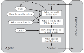
- Agents and Environments
- Agents
- An agent exists and performs intelligent behaviors,
e.g., makes decisions and takes actions, in a specific
environment and interacts with that environment via
a sense-understand-plan-act loop, i.e.,
- An agent perceives its environment through
sensors, e.g., camera, touch, taste, keyboard
input; these sensors provide percepts, which
form percept sequences over time.
- Agents act in their environment through
actuators, e.g., limbs, tools, allowable moves in
a game; actuators perform actions that can
modify the environment (including the agent's
internal state and/or position in the environment).
- An agent's choice of action is specified as an
agent function and implemented as an agent
program relative to a particular architecture.
- Agent functions are also known as policies
and there are various names for agent
programs depending on the application, e.g.,
controllers (robotics).
- In general, an agent's action-choice can
depend on its entire percept-history to
date; however, we will in this course
focus an agents whose action-choices
depend on the current percept.
- There are typically many ways to implement
an agent function, e.g., lookup tables,
IF-THEN statement blocks, neural networks.
- An agent may have knowledge about its environment,
e,g., environment model, game rules / allowable
moves.
- EXAMPLE: Some example agents:
- Roomba vacuum cleaner
- Human players in a game of chess
- Self-driving vehicle
- AI personal assistant
What are the sensors, percepts, actuators, actions, and
knowledge (if any) associated with each of these agents?
- An agent may have multiple internal states, with
percept / action pairs between these states
encoded in a state-transition function.
- EXAMPLE: Three deterministic finite-state agents that
operate in a 2D grid-world (Wareham and Vardy (2018)).
- State transitions are specified as (state, percept,
action, state) tuples, where an action is
specified as an (environment-change, agent move)
pair.
- Agent processing starts in state q0.
- What does each of these agents do?
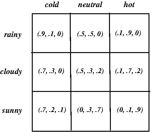
- EXAMPLE: A stochastic agent
- Specified as a table whose x- and y-axes are
percepts and table entries are probability-vectors
specifying the probabilities of a set of actions
relative to a set of x/y-percept combinations.
- Consider the following agent which specifies the
probabilities of
what to do (wear coat, carry umbrella, do nothing
extra) if you want to take a walk outside
depending on the weather ((rainy / cloudy / sunny)
x (cold / neutral / hot)):
- A rational agent does the best possible action
at each point wrt optimizing some pre-defined
performance measure; such an agent has an optimal
policy.
- Note that rationality is NOT omniscience, i.e.,
knowing the complete environment and the
outcomes of all (even random) actions.
- EXAMPLE: Going across street at crosswalk to
see friend vs not crossing street
because of incoming meteor from space.
- Four basic types of agents:
- Simple reflex agents
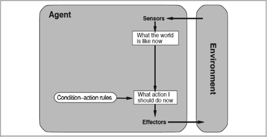
- This simplest type of agent reacts without
understanding or planning by using
sets of encoded IF-THEN rules that
directly link percepts and actions, e.g.,
the deterministic finite-state and
stochastic agents given above.
- The intelligence encoded in such agents
can be impressive, e.g., Brooks' Genghis
robot, basic obstacle avoidance in
self-driving vehicles, but are ultimately
limited in that there is little understanding
or planning in the action-selection process.
- Model-based agents
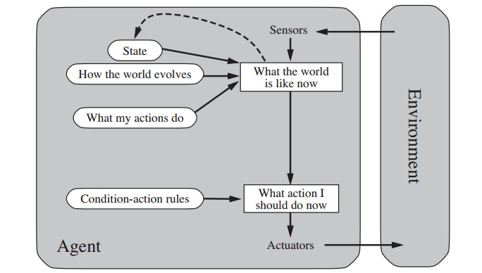
- This type of agent maintains a non-trivial
internal state that incorporates knowledge
of how the world works and a model of the
world encountered to date (including the
agent's own past actions in the world, e.g.,
the two-state deterministic finite-state
agent given above).
- The intelligence encoded in such agents now
allows understanding to be part of the
action-selection process.
- Goal-based agents
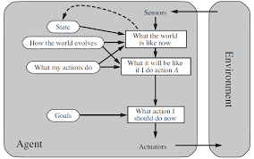
- This type of agent incorporates a description
of an agent's wanted goal, e.g., the
destination to be reached, as well as a
way of evaluating if that goal has been
achieved, e.g., are we at the requested
destination?
- Typically more complex than simple reflex
agents but much more flexible in terms of
the intelligence it can encode (in particular,
planning as part of the action-selection
process).
- Utility-based agents
- This type of agent incorporates a utility
function that internalizes some performance
measure, e.g., the distance traveled on
a particular path from the start point to
the destination, and is thus capable of
optimizing this performance measure, e.g.,
choosing the shortest path from a start
point to the destination.
- Such agents are more complex still but can
(given an appropriate utility function)
encode general rationality.
- Note that choosing the appropriate utility
function is crucial to the encoded degree
of rationality and this is typically
very hard to do.
- The intelligence in the four types of
agents above is hard-coded using hand-crafted
algorithms.
The most complex type of agent can learn from
experience and both become rational and
maintain this rationality in the face of changing
environments. The resulting agent programs
are machine-crafted and will be discussed in
the final lectures of this course.
Thursday, September 12 (Lecture #3)
[ DC3200, Lecture #2 and
DC3200, Lecture #3;
RN3, Chapters 2 and 3; Class Notes]
- Agents and Environments (Cont'd)
- Environments
- The current configuration of an environment is that
environment's current state.
- A configuration encodes all entities in an
environment, including the agents (and, if
applicable, the positions and internal states
of these agents) within the environment.
- EXAMPLE: A configuration of a Solitaire card
game would show all cards and their order,
both in the visible stacks of cards and the deck
of undrawn cards.
- What an agent perceives may not be a complete
representation of an environment's state;
however, such observations are all the agent
has to make its decisions.
- EXAMPLE: An agent playing a game of Solitaire can
only see the visible stacks of cards and their
orders in these stacks.
- Environments can be viewed as problems to which agents
provide solutions, e.g., a path between locations on a
map, a sequence of rule-applications that results in a
wanted goal.
- EXAMPLE: Some example agents:
- Roomba vacuum cleaner
- Human players in a game of chess
- Self-driving vehicle
- AI personal assistant
What are the environments, environment configurations,
and problems associated with each of these agents?
- Environments have associated state and action spaces.
- State space = the number of possible
configurations of the environment.
- Action space = the number of possible actions
relative to a state.
- Average / worst-case measures of the sizes of
state and action spaces are frequently used as
measures of environment complexity.
- Are good measures of the computational
complexity of searching state / action
spaces by exhaustive search.
- EXAMPLE: State space sizes for some games
- Tic-Tac-Toe: 10^4
- Chess: 10^{43}
- Go: 10^{172}
- EXAMPLE: Total # sequences of actions in some game
(game tree complexity)
- Tic-Tac-Toe: <= 10^5
- Chess: <= 10^{123}
- Go: <= 10^{360}
- Starcraft II: > 10^{1000)
- Given that there are approximately 10^{80} atoms
in the universe and these atoms are expected to
decay into a quark mist in 10^{70} years, the
opportunities for completing exhaustive searches
for the largest state spaces are severely limited;
that is why you need the smartest search algorithms
possible (some of which we will be looking at
over the next several lectures).
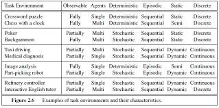
- Environments have several properties:
- Fully vs partially observable by agent, e.g.,
chess vs poker.
- Deterministic vs stochastic from viewpoint
of agent, e.g., chess vs poker.
- Episodic vs sequential, i.e., next episode does not
or does depend on previous episodes, e.g., OCR
(Optical Character Recognition) vs chess.
- Static vs dynamic, i.e., environment changes
discretely when agents act or continuously
(possibly even during agent decision), e.g.,
turn-based (chess) vs real-time (Starcraft) games.
- Discrete vs continuous conception of time and
environment change, e.g., poker /chess vs
self-driving vehicles.
- Single agent vs multiple agents, e.g., Solitaire
vs chess vs self-driving vehicles.
- Complete vs incomplete knowledge of actions and
their consequences, e.g., chess vs real life.
- Example environments and their properties:
- EXAMPLE: Some example agents:
- Roomba vacuum cleaner
- Human players in a game of chess
- Self-driving vehicle
- AI personal assistant
What are the properties of the environments associated
with each of these agents?
- The properties of an environment dramatically affect
the computational difficulties of designing agents for
and operating agents within environments; we will see
this in action over the course of our lectures, many
of which will consider only the simplest environments..
- Potential exam questions
- Problem-solving and search
- Problem-solving agents are rational agents that act in
environments to solve the problems posed by those
environments.
- In the simplest case, they are goal-based agents
that find a sequence of actions that satisfies
some goal, e.g., find a path from a start point to
a given destination.
- More complex cases involve utility-based agents
that find a goal-achieving sequence of actions
that optimize some performance measure, e.g., find
a shortest path (in terms of distance
traveled) from a start point to a specified
destination.
- EXAMPLE: Finding a (shortest) path from our
classroom at MUN to the Winners store at the
Avalon Mall.
- A solution (also known as a solution path) is
a sequence of actions that terminates in the
problem's goal.
- A well-defined problem consists of:
- An initial state that the agent starts in.
- The actions possible from each state.
- Specified as a successor function, e.g.,
from position (x,y) in a 2D grid-based maze,
you can go up, down, left, or right.
- This is typically refined relative to each
state to the viable actions for that state,
i.e., the actions that do not violate
constraints like moving into a wall in a
2D maze.
- The set of goal states
- Specified as a goal test function that returns
"Yes" if a given state is in the set of goal
states and "No" otherwise, i.e., are we
just outside the main door of the Winners
store at the Avalon Mall? Is our chess
opponent in checkmate?
- Action cost function
- Most problems assume positive non-zero
action costs.
- The cost of a solution is the sum of the costs
of the actions in that solution's associated path;
an optimal solution has the lowest cost over all
possible solutions.
- EXAMPLE: Shortest path between two vertices in an
edge-weighted graph G.
- Problem definition:
- Start vertex in G.
- For each vertex v in G, the set of edges
with v as an endpoint.
- Destination vertex in G.
- Edge-weight function for G.
- The problem objective is to find a shortest (in
terms of summed edge-weights) path in G from the
start vertex to the destination vertex.
- EXAMPLE: Shortest path between two locations in a
2D grid G incorporating obstacles.
- Problem definition:
- Start location in G.
- For each location l in G that is not part of an
obstacle, the subset of possible moves
{up, down, left, right} that do not land on
some obstacle when executed at l.
- Destination location in G.
- Function that assigns cost 1 to up, down,
left, and right moves.
- The problem objective is to find a shortest (in
terms of # of moves) path in G from the
start location to the destination location.
- EXAMPLE: Most efficient plan for making a cup of tea.
- Problem definition:
- State consisting of {cup(empty), teaBag,
kettle(empty), faucet, electricity}.
- The set A of actions, i.e.,
- kettle(empty) + faucet => -kettle(empty) +
kettle(fullCold)
[fill kettle with cold water]
- cup(empty) + faucet => -cup(empty) +
cup(fullCold)
[fill cup with cold water]
- kettle(fullCold) + electricity =>
-kettle(fullCold) + kettle(fullHot)
[boil kettle]
- cup(fullCold) + electricity =>
-cup(fullCold) + cup(fullHot)
[boil cup]
- cup(empty) + teaBag => -teaBag +
-cup(empty) + cup(teaBag)
[add tea bag to cup]
- cup(empty) + kettle(fullHot) =>
-cup(empty) + cup(fullHot)
[add hot water to cup]
- cup(teaBag) + kettle(fullHot) =>
-cup(teaBag) + cup(tea)
[make tea I]
- cup(fullHot) + teaBag =>
-cup(fullHot) + -teaBag + cup(tea)
[make tea II]
Each action X => Y (where X is the cause
and Y is the consequence) is an IF-THEN
rule whose application to a state s is viable
if for each x (-x) in X, x is (not) in s and
results in a state s' that modifies s by
adding (removing) each y to (from) s such that
y (-y) is in Y, e.g., the initial state is
modified to state s' = {cup(teaBag),
kettle(empty), faucet, electricity} by the
application of action 5.
Given the above, for each possible state s
that is a subset of {faucet, electricity,
kettle(empty), kettle(fullCold),
kettle(fullHot), teaBag, cup(empty),
cup(fullCold), cup(fullHot), cup(teaBag),
cup(tea)}, the set of viable actions for s is the
subset of A that can be viably applied to s.
- Any state including {cup(tea)}.
- Function that assigns cost 1 to each action.
- The problem objective is to find a most efficient
(in terms of # of actions) plan that, starting in
the initial state, creates a hot cup of tea.
- The formalism above is a simplified version of
the input language for the STRIPS (STanford
Research Institute Problem Solver) automated
planning system (Fikes and Nilsson (1971); see
also Bylander (1994)) and will be used in Assignment #2.
- The type of state in this problem has what is
known as a factored representation, i.e.,
a state with a
multi-component internal structure; we will be
using this type of problem-state frequently
later in the course.
Tuesday, September 17 (Lecture #4)
[DC3200, Lecture #3;
RN3, Chapter 3; Class Notes]
- Problem-solving and search (Cont'd)
- Search is the process of exploring a problem's search
space to find a solution. This process generates a
search tree in which the root node, edges, and
non-root nodes correspond to the initial problem
state, actions, and possible solution paths.
- Starting with the root node, the search tree is
generated by expanding nodes, i.e., generating
the nodes reachable from a node n by viable actions,
in some specified manner until either a goal
node is found or it is established that no
goal-state is reachable by any sequence of actions
starting at the root node.
- At each point in this process, the list of
leaf nodes that has been generated but
not yet expanded is known as the fringe.
- Search algorithms can be distinguished in
how they select nodes from the fringe to
expand.
- Each search tree node corresponds to problem
state; however, if actions are reversible,
a problem state can be associated with multiple
search tree nodes and a finite-size problem state
space can have an infinite-size search tree.
- EXAMPLE: Search tree for problem of finding a
shortest path between two vertices in a graph.
[DC3200, Lecture #3, Slides 14-26
(PDF)]
- EXAMPLE: Search tree for 15 puzzle
[DC3200, Lecture #3, Slides 27-28
(PDF)]
- Must distinguish problem-states and search-tree
nodes - the former are configurations of the
problem environment and the latter are bookkeeping
data structures allowing recovery of solution
paths to goals. To this send, a search tree node
n typically contains the following data:
- The problem state associated with n.
- A pointer to n's parent node, i.e., the node
whose expansion generated n.
- The action by which n was generated from its
parent node.
- The cost of the sequence of actions on the
path in the search tree from the root node
to n.
- This is traditionally denoted by g(n).
- The depth of n, i.e., the number of actions on
the path in the search tree from the root node
to n.
Additional data may also be stored in the node
depending on the search algorithm used.
- ALGORITHM: General uninformed tree search
1.   Function Tree-Search(problem, strategy)
2.     fringe = {Node(problem.initial_state)}
3.     while (true)
4.       if (fringe.empty) return fail
5.       node = strategy.select_node(fringe)
6.       if (node.state is goal) return solution
7.       else fringe.add(Expand(node, problem))
- ALGORITHM: Node expansion [ASSIGNMENT #1]
1.   Function Expand(node, problem)
2.     successors = {}
3.     for a in viablActions(problem.actions, node)
4.       s = Node(node.state.do_action(a))
5.       s.parent = node
6.       s.action = a
7.       s.g = node.g + s.action.cost
8.       s.depth = node.depth + 1
9.       successors.add(s)
10.    return succesors
- We will build on these algorithms below when we
consider different search strategies.
Search strategies
- Measures for assessing the problem-solving performance
of a search-strategy algorithm s:
- Completeness, i.e., is s guaranteed
to find a solution if it exists?
- Optimality, i.e., is s guaranteed
to find an optimal solution?
- Time complexity, i.e., how long does it take for
s to find a solution or establish that a solution
does not exist?
- Measures the total number of search tree nodes
generated.
- Space complexity, i.e., how much memory is needed
to execute s?
- Measures the maximum number of search tree
nodes that must be stored at any point in the
search process.
Aspects of the search tree typically used to derive
time and space complexity functions are the branching
factor b (the maximum number of successor nodes for
any tree node) and the depth d (of the shallowest
goal node, if a solution exists, and the maximum depth
of a generated node, if one does not). Note that the
size of a search tree is upper-bounded by b^{d+1}.
- Two categories of search strategies:
- Uninformed (blind) search
- Has no extra information about states in a
search tree beyond that in the problem
description, i.e., algorithm operations
limited to successor, generation, and
goal test.
- Informed search
- Has extra information which allows
guesses about which states are more
likely to be on useful / optimal
solution paths, i.e., algorithm operations
additionally include the value of heuristic
node evaluation function h(n).
- Hopefully leads to faster search.
We will look first at uninformed search strategies
and then move on to informed search strategies, with
an intermediate stop to consider closed lists, a
key algorithmic technique for optimizing the
performance of both types of search strategies.
Uninformed (blind) search strategies
- Breadth-First Search (BFS)
Lines modified from the algorithm for general
uninformed tree search are indicated by "<=".
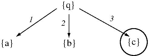
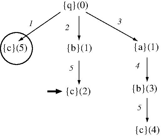
- EXAMPLE: BFS for a shortest (# edges) path between
vertices A and C in an unweighted graph.
[DC3200, Lecture #3, Slides 44-48
(PDF)]
- EXAMPLE: BFS for a shortest (Manhattan distance) path between two
locations in a 2D grid with obstacles
[DC3200, Lecture #3, Slides 49-54
(PDF)]
- EXAMPLE: BFS for a shortest (summed
action-cost) solution to a modified
STRIPS planning problem based on facts
[q, a, b, c], initial state [q], goal state
[c], and actions
- q => -q + a (cost 1)
- q => -q + b (cost 1)
- q => -q + c (cost 1)
- a => -a + b (cost 1)
- b => -b + c (cost 1)
- Performance of BFS
- BFS is complete.
- BFS can explore the entire search tree;
hence, if there is a goal node
in the tree, BFS will find it.
- Note that if there are multiple
goal nodes in the search tree,
BFS will find the shalowest one.
- BFS is not optimal in general.
- This is because the path to the
shallowest goal node need not
have the optimal cost.
- EXAMPLE: BFS is not optimal for finding a
shortest (summed edge-weights) path between vertices A and C in an
edge-weighted graph.
[DC3200, Lecture #3, Slide 57
(PDF)]
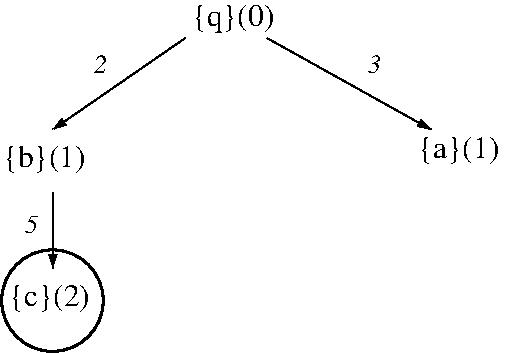
- EXAMPLE: BFS is not optimal in finding a
shortest (summed action-cost) solution to a modified
STRIPS planning problem based on facts
[q, a, b, c], initial state [q], goal state
[c], and actions
- q => -q + c (cost 5)
- q => -q + b (cost 1)
- q => -q + a (cost 1)
- a => -a + b (cost 2)
- b => -b + c (cost 1)
- BFS is optimal if (1) path costs
never decrease as depth increases
or (2) all action costs are the
same.
- Time Complexity: O(b^{d+1}), as all nodes
in a search tree of depth d with
branching factor b may be generated.
- Space Complexity: O(b^{d+1}), as all
generated nodes must be stored in
memory to allow reconstruction of
solution paths from goal nodes via
parent pointers.
Uniform Cost Search (UCS)
Lines modified from the algorithm for general
uninformed tree search are indicated by "<=".
EXAMPLE: UCS for a
shortest (summededge-weights) path between vertices A and C in an
edge-weighted graph.
[DC3200, Lecture #3, Slide 57
(PDF)]
EXAMPLE: UCS for a shortest (summed
action-cost) solution to a modified
STRIPS planning problem based on facts
[q, a, b, c], initial state [q], goal state
[c], and actions
- q => -q + c (cost 5)
- q => -q + b (cost 1)
- q => -q + a (cost 1)
- a => -a + b (cost 2)
- b => -b + c (cost 1)
Performance of UCS
- UCS is complete
- UCS is optimal if action costs > 0 (epsilon)
- Time Complexity: O(b^{1 +
floor(C*/epsilon)}), where C* is the
cost of an optimal solution
- This is necessary because path
cost is no longer linked to
depth.
- Can be much bigger than b^{d+1} is the
worst case.
- Space Complexity: O(b^{1 +
floor(C*/epsilon)})
Thursday, September 19 (Lecture #5)
[DC3200, Lecture #3;
RN3, Chapter 3; Class Notes]
- Problem-solving and Search (Cont'd)
- Uninformed (blind) search strategies (Cont'd)
- Depth-First Search (DFS)
Lines modified from the algorithm for general
uninformed tree search are indicated by "<=".
- ALGORITHM: DFS (recursive)
1.   Function DFS(node, problem)
2.     if (node.state is goal) return solution
3.     successors = Expand(node, problem)
4.     for (s in successors):
5.       DFS(s, problem)

     Call DFS(root_node, problm)
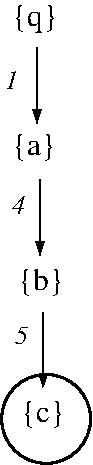
- EXAMPLE: DFS for a solution to a modified
STRIPS planning problem based on facts
[q, a, b, c], initial state [q], goal state
[c], and actions
- q => -q + c (cost 1)
- q => -q + b (cost 1)
- q => -q + a (cost 1)
- a => -a + b (cost 1)
- b => -b + c (cost 1)
- Performance of DFS
- DFS is not complete in general
- Can enter infinite loop if does
not keep track of already-visited
states.
- EXAMPLE: DFS for a
path between vertices A and B in an
unweighted graph.
[DC3200, Lecture #3, Slide 57
(PDF)]
- Infinite loops can be prevented
by algorithm
enhancements (see DLS and ID-DFS
below) or by the
use of closed lists (see below).
- DFS is not optimal in general
- This is because it returns the
first goal found.
- EXAMPLE: If B is visited before D, DFS is
not optimal for finding a shortest (summed
edge-weight) path between vertices A and C
in an
edge-weighted graph.
[DC3200, Lecture #3, Slide 57
(PDF)]
- EXAMPLE: DFS is not optimal for
finding a shortest (either # moves
or summed action-cost) solution to
the modified STRIPS planning
problem given above.
- Time Complexity: O(b^m), where m is
is the depth of the deepest node.
- Space Complexity: O(bm)
- This is because in the worst case,
DFS stores a path of m nodes from
the route along with the b
successors of each node on this
path.
- Depth-Limited Search (DLS)
- Solves the infinite-loop DFS problem by
limiting the maximum search depth to some
L > 0.
- ALGORITHM: DLS (recursive)
1.   Function DLS(node, L, problem)
2.     if (node,depth > L) return "cutoff"       <=
3.     if (node.state is goal) return solution
4.     successors = Expand(node, problem)
5.     for (s in successors):
6.       DLS(s, L, problem)

     Call DLS(root_node, L, problm)
Lines modified from the algorithm for DFS
(recursive) are indicated by "<=".
- Performance of DLS
- DLS is not complete
when solution depth > L
- DLS is not optimal in general
- This is because it returns the
first goal found.
- Time Complexity: O(b^L)
- Space Complexity: O(bL)
Iterative Deepening Depth-First Search (ID-DFS)
- In DLS, one chooses maximum search depth L
by analysis of the problem's state space;
alternatively, one can gradually increase
the depth limit until a solution is found.
This is what ID-DFS does.
- ALGORITHM: ID-DFS
1.   Function ID-DFS(node, , problem)
2.     for d in (1,infty)
3.       result = DLS(node, d, problem)
4.       if (result != "cutoff") return result
Performance of ID-DFS
- ID-DFS is complete
- ID-DFS is optimal under same conditions
as BFS
- Time Complexity: O(b^{d+1}), where d is the
depth of the shallowest goal node
- As nodes may be recomputed as
L is increased, may seem wasteful;
however, in practice, generates
about twice as many nodes as BFS.
- Space Complexity: O(bd)
As it combines the advantages of both BFS and
DFS, ID-DFS is in general preferable to both
BFS and DFS.
TABLE: Uninformed search strategy comparison
[DC3200, Lecture #3, Slide 79
(PDF)]
INTERLUDE: A look at the mechanics of
Assignment #1.
- How do you modify the BFS, UCS, and DFS
(non-recursive) algorithms above to
print all solutions to a given
problem?
None of the algorithms presented above remember the
states that have already been expanded. Such states
lead to duplicated effort and (if actions are
reversible) infinite loops.
Such states can be remembered and avoided using
closed lists, which are lists of previously expanded
(and hence explored) nodes.
- To ensure efficient lookup, closed lists are often
implemented using dictionaries and hash tables
(the latter of which will be described in detail
in several lectures).
In addition to eliminating infinite loops, such
lists can lead to an exponential savings in the
number of nodes generated; however, these lists
are not universal cures for all of the ills that
can plague search
(see below).
Following terminology in Russell and Norving, tree
search algorithms that use closed lists (1) rename
fringe lists as open lists and, perhaps more
confusingly, (2) are renamed graph search algorithms
(after the classic BFS graph search algorithm that
implements closed lists implicitly using a node
coloring scheme to avoid re-exploring
previously-encountered vertices).
ALGORITHM: General uninformed graph-based search
1.   Function Graph-Search(problem, strategy)
2.     closed = {}                                 <=
3.     open = {Node(problem.initial_state)}
4.     while (true)
5.       if (fringe.empty) return fail
6.       node = strategy.select_node(open)
7.       if (node.state is goal) return solution
8.       if (node.state in closed) continue        <=
9.       closed.add(node.state)                    <=
10.      open.add(Expand(node, problem))
Lines modified from the algorithm for general
uninformed tree search are indicated by "<=".
ALGORITHM: Graph-based BFS
1.   Function gbBFS(problem)
2.     closed = {}                                 <=
3.     open = Queue{Node(problem.initial_state)}
4.     while (true)
5.       if (fringe.empty) return fail
6.       node = open.pop()
7.       if (node.state is goal) return solution
8.       if (node.state in closed) continue        <=
9.       closed.add(node.state)                    <=
10.      open.add(Expand(node, problem))
Lines modified from the algorithm for (tree-based) BFS
are indicated by "<=".
ALGORITHM: Graph-based DFS
1.   Function gbDFS(problem)
2.     closed = {}                                 <=
3.     open = Stack{Node(problem.initial_state)}
4.     while (true)
5.       if (fringe.empty) return fail
6.       node = open.pop()
7.       if (node.state is goal) return solution
8.       if (node.state in closed) continue        <=
9.       closed.add(node.state)                    <=
10.      open.add(Expand(node, problem))
Lines modified from the algorithm for (tree-based) DFS
are indicated by "<=".
Graph-based search algorithms still generate search
trees; however, as each problem state can now only
label only one search tree node, the search tree is
effectively overlaid on the state-space graph whose
vertices correspond to problem states and arcs
correspond to actions linking pairs of states.
- Problem states may repeat in the fringe data
structure, as states may be encountered several
times before they are expanded and added to the
closed list.
EXAMPLE: Operation of gbBFS in finding
a shortest (# edges) path between vertices A and C in
a graph. [txt]
EXAMPLE: Operation of gbDFS; in finding a path between
vertices A and C in a graph.
[txt]
Performance of a graph-based version of search
strategy s
- Completeness is as in the tree-based version of s.
- Optimality depends on s.
- As graph-based search effectively discards
all paths to a node but the one found first,
it is only optimal if we can gaurantee that
the first solution found is the optimal
one, e.g., BFS or UCS with all actions having
the same cost.
- Time Complexity: O(#states)
- This is because each state is expanded
at most once and in the worst case,
every state in the environment must be
expanded; hence, it is the same for
every search strategy.
- In practice, the actual number of generated
states is far lower than this worst case.
- Space Complexity: O(#states)
- This is because of the closed list.
- Note that this also applies to tree-based
versions that ran in linear space, e.g., DFS
and its associated variants.
Tuesday, September 24 (Lecture #6)
[DC3200, Lecture #5;
RN3, Chapter 3; Class Notes]
- Problem Solving and Search (Cont'd)
- Informed (heuristic) search strategies
- Uses problem-specific knowledge encoded as
heuristic functions that (ideally, but not
always) cut down the total number of nodes
searched and speed up search times to goal.
- Heuristic function h(n) gives a (hopefully
good) estimate of the cost of the optimal
path from node n to a goal node. If n is a
goal node, h(n) = 0.
- h*(n) = perfect heuristic which gives exact
cost of optimal path from n to goal node
(and wouldn't that be nice ...)
- EXAMPLE: A heuristic h1(n) for shortest-path in
edge-weighted graphs is the cost of the
lowest-cost edge
originating at n that does not double back to
an already-explored node.
- EXAMPLE: A heuristic h2(n) for shortest-path in 2D
grids is the Manhattan distance from n to the
the requested location.
- EXAMPLE: A heuristic h3(n) for efficient plans to
make tea is the modified Hamming distiance from
the problem state n to a possible goal state.
- Replace all non-specified items in the goal
by * to generate pg and then compute the
Hamming distance between the non-star
positions in pg and the state encoded in n.
- For example, given a goal p1 + -p3 + p4 in
a five-item state, pg = 1*01* and the
modified Hamming distance from pg to
sn = 01000 is 2 (position 3 matches and
positions 1 and 4 do not match).
- Types of heuristics
- An admissible heuristic never
overestimates the distance from a node
n to a goal node, i.e., h(n) <= h*(n ).
- Can be seeen as an optimistic guess.
- When h() is admissible, f(n) = g(n) +
h(n) never overestimates the cost
of a best-possible path from the initial
state to a goal state that goes
through n.
- A consistent heuristic (also called a
monotone heuristic) has
|h(a) - h(b)| <= c(a,b), where c(a,b) is the
optimal cost of a path from a to b.
- With such a heuristic, the difference of
the heuristic values of two nodes must
be less than or equal to the optimal
cost of a path between those nodes.
- Every consistent heuristic is also
admissible; indeed, it is hard (but not
impossible) to construct an admissible
heuristic that is not consistent.
- When h(n) is consistent, the values
of f(n) = g(n) + h(n) along any
path are non-decreasing; this will turn
out to be very useful later in our
story.
- EXAMPLE: Which of the heuristics h1(n), h2(n),
and h3(n) above are admissible? Which are
also consistent?
- Informed search strategies differ in how they
combine g(n) and h(n) to create a function
f(n) that is used to select the next node
in the open list to expand.
- Tree-based Greedy Best-First BFS (GBeFS)
- Select node in open list with
lowest f(n) value, where f(n) = h(n),
i.e., only cares about distance to goal.
- Resembles DFS in that it tries a single
path all the way to the goal and backs
up when it hits a "dead end".
- EXAMPLE: BFS vs GBeFS in shortest-path in 2D
grid world with obstacles.
[DC3200, Lecture #5, Slides 19-33
(PDF)]
- ALGORITHM: Tree-based GBeFS
1.   Function GBeFS(problem, h(n))
2.     open = PriorityQueue{f(n) = h(n)}                   <=
3,     open.add(Node(problem.initial_state))
f.     while (true)
5.       if (open.empty) return fail
6.       node = open.min_f_value()                         <=
7.       if (node.state is goal) return solution
8.       else open.add(Expand(node, problem))
Lines modified from the algorithm for UCS
are indicated by "<=".
- Performance of GBeFS (similar to DFS)
- GBeFS is not complete
- May not find goal; may even "get
lost" and retrace paths if
heuristic is bad.
- GBeFS is not optimal
- Time Complexity: O(b^m), where m =
maximum explored node depth.
- Space Complexity: O(bm)
- Though performance not so great in general,
performs well for carefully crafted
heuristics; such heuristics can be derived
using means-ends analysis.
- GBeFS was the core search strategy underlying
the earliest automated reasoning systems
Logic Theorist (1956) (Newell and Simon
(1956)) and GPS (General Problem Solver
(1959) (Newell, Shaw, and Simon (1959)) as
well as foundational computational modeling
work on problem solving by humans
(Newell and Simon (1972)).
- Problem Solving and Search (Cont'd)
- Informed (heuristic) search strategies (Cont'd)
- Tree-based A* search
- Most well-known BeFS algorithm.
- Select node in open list with
lowest f(n) value, where f(n) = g(n) + h(n),
i.e., cares about total distance from
start state to goal.
- ALGORITHM: Tree-based A* search
1.   Function A*(problem, h(n))
2.     open = PriorityQueue{f(n) = g(n) + h(n)}            <=
3,     open.add(Node(problem.initial_state))
f.     while (true)
5.       if (open.empty) return fail
6.       node = open.min_f_value()                         <=
7.       if (node.state is goal) return solution
8.       else open.add(Expand(node, problem))
Lines modified from the algorithm for UCS
are indicated by "<=".
- Performance of Tree-based A*
- Tree-based A* is complete
- Will eventually visit all nodes
in the search tree, starting with
those who h-values are lowest.
- Tree-based A* is optimal if h(n) is admissible
- Time Complexity: O(b^m), where m =
maximum explored node depth.
- Space Complexity: O(bm)
- Graph-based A* search
- Let us now try to optimize the runtime of
A* search by using closed lists.
- ALGORITHM: Graph-based A* search
1.   Function gbA*(problem, h(n))
2.     closed = {}                                         <=
3.     open = PriorityQueue{f(n) = g(n) + h(n)}
4,     open.add(Node(problem.initial_state))
5.     while (true)
6.       if (open.empty) return fail
7.       node = open.min_f_value()
8.       if (node.state is goal) return solution
9.       if (node.state in closed) continue                <=
10.      closed.add(note.state)                            <=
11.      open.add(Expand(node, problem))
Lines modified from the algorithm for
tree-based A* search are indicated by "<=".
- Performance of Graph-based A*
- Graph-based A* is complete
- Graph-based A* is optimal if h(n) is consistent
- Admissible heuristics do not
suffice for optimality, as
"raw" graph-based search only
retains the first-encountered path
to a repeated state (where a
later-encountered path may be
better).
- If a consistent heuristic is used,
the values of f(n) along any path
are non-decreasing; as the
sequence of nodes expanded by
graph-based A* is in non-decreasing
order of f(n), any node selected
for expansion is on an optimal
path as all later nodes are at
least as expensive!
- Time Complexity: O(b^m)
- Space Complexity: O(b^m)
- EXAMPLE: (VERY detailed) Graph-based A* search
for path between two locations in a 2D grid
with obstacles
[DC3200, Lecture #5, Slides 68-147
(PDF)]
- Graph-based A* also has the property that
no other optimal uninformed search algorithm
can expand fewer nodes; that being said, the
number of nodes that need to be searched and
retained (as part of the closed list) is
still exponential in the worst case and can
be prohibitive in practice.
Potential exam questions
There are a variety of ways of improving the performance in
practice (though not in the worst case) of the search
algorithms above; these ways tend to be specific to
particular types of environments, e.g., 2D grids
(see DC3200, Lecture #7), or search algorithms, e.g.,
graph-based A* search (see DC3200, Lecture #5).
An important example of the latter is using appropriate data
structures to optimize membership query time in open and
closed lists in graph-based search. Some common data
structures and their worst-case membership query times for
an open / closed list with n items are:
- List /array: O(n)
- Set / dictionary (via balanced search trees): O(log n)
- Hash table: O(n)
- Perfect hash table: O(1)
Given their simplicity and the possibility of O(1) membership
query time, it is worth looking at hash tables and the
manners in which they can be made as perfect as possible.
Hash Tables: Overview and Implementation
- A hash table is at its heart a 1D array that stores
instances of more complex data structures for easy
lookup.
- A commonly-stored data structure is key-value
pairs.
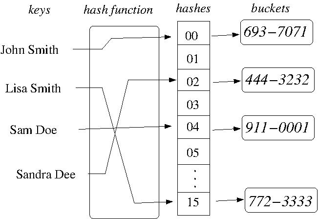
- EXAMPLE: A hash table for person name / phone number
pairs with 16 buckets.
- Given a data structure d, a hash function is used to
compute an integer that is d's (initial) position in the
hash table (also called d's bucket). Such functions are
made as simple as possible to optimize membership query
time.
- As keys are typically less
complex than their associated values, the hash
function is applied to the key and the full
key / value pair is stored in the bucket.
- In a perfect hash table (see example above), each data
structure maps to a
unique position in the hash table (giving O(1)
membership query time if the hash function is simple
enough).
- If two or more data structure map to the same
position, i.e., a hash collision has occured, an
appropriate collision resolution policy is used to
redistribute the colliding items in the hash table such
that membership query time is degraded as little as
possible.
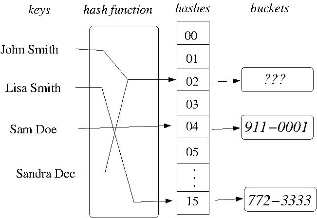
- EXAMPLE: A hash collision in a hash table for
person name / phone number pairs with 16 buckets.
Hash functions
- Have many uses in addition to hash tables, e.g.,
password protection, data verification (checksum
creation), proximity queries in computational geometry
(geometric hashing).
- Hash functions typically have an associated input
format and range of input values; if a hash function is
applied to an unexpected value or a value outside the
given range, the results may be poor or undefined.
- EXAMPLE: Hashing a character string to an integer.
[DC3200, Lecture #6, Slide 18
(PDF)]
- Output ranges, i.e., the available storage indices in a
hash table, can be ensured by the modulus operator.
- Hash function properties
- There a variety of properties a hash function
can have, whose necesssity depends on the
application, e.g.,
- Determinism (A good hash function should
always produce the same output for
the same input)
- Uniformity (a good hash function maps inputs as
evenly as possible over its output range to
prevent hash collisions)
- Data Normalization (Ignores irrelevant features
of the input, e.g., upper / lower case
letters; is application-dependent, e.g.,
data lookup (good) vs password protection
(bad)).
- Continuity (Small changes in the input have
small changes in the output; is
application-dependent, e.g., geometric
hashing (good) vs password protection
(bad))
- Reversibility / invertibility (input can be
easily recovered from the output; is
application-dependent, e.g., geometric
hashing (good) vs password protection
(bad))
- One can also characterize hash functions in terms
of purely mathematical properties, e.g.,
- Injective (Every input maps to a unique
output, i.e., the function is one-to-one)
- Note that some outputs may not be mapped.
- (Many) Injective functions are
invertible.
- Such functions are perfect hash
functions!
- Surjective (Every output has at least input
that maps to it, i.e., the function is onto)
- (Many) Surjective functions are not
invertible.
- Bijective (Every input maps to a unique output
and every output maps to a unique input,
i.e., the function is one-to-one and onto)
- Such functions are minimal perfect
hash functions, i.e., they are perfect
hash functions with the
smallest-possible associated hash
tables!
- EXAMPLE: Diagrams of injective, surjective and
bijective functions
[DC3200, Lecture #6, Slide 40
(PDF)]
- Hash function algorithms
- Simple hash functions
- Trivial hashing: When (typically small) data
can be directly translated to its hash
value, e.g., h(ASCII character) = ASCII
character code.
- Modulus hashing: h(x) = x mod n
- Only applicable to integers
- Focuses on lower-order bits in given
integer; truncates higher-order bits.
- Can have uniformity problems if x is not
a multiple of n.
- Binning hashing: h(x) = x / n
- Only applicable to integers
- Focuses on higher-order bits in given
integer; truncates lower-order bits.
- Uniformity characteristics almost the
opposite of modulus hashing.
- String hashing
- Character summation hashing: Sum the ASCII /
Unicode values of the characters in the
string.
- Block summation hashing: Treat each succesive
block of n characters as a single long
integer whose bits are the concatenated
ASCII / Unicode codes for those characters
and sum the long integers corresponding to
all character-blocks.
- EXAMPLE: What are the characteristics of
both of these schemes wrt -jectivity,
uniformity, invertibility, and input
character order?
- Geometric hashing
- Converts n-dimensional location input
(x1, x2, ..., xn) into an integer.
- For a 2D grid with width wd and height ht,
n(x,y) = (y * wd) + x; note that this
h() is a minimal perfect hash function
whose output i is invertible (y = i / wd,
x = i % wd).
Hash collisions: Overview and Resolution Policies
- Collision resolution is expensive and should be
avoided where possible.
- Perfect (injective) hash functions ensure that there
are no collisions; however, this requires that the
input space is smaller than the hash table, which
is seldom the case -- indeed, the input space is
typically MUCH larger than the hash table.
- If one is forced (as one typically is) to use imperfect
hash functions, the probability of a collision
rises surprisingly fast with each new hash.
- The probability of a hash collition after n hashes
with a uniform hash function into a hash table
with m buckets is 50% when n is approximately
sqrt(m).
- EXAMPLE: The Birthday Paradox
- The probability of two people having the
same birthday is 50% when there are only
23 people!
- This is effectively the probability of a
hash colision when hashing n = 23 (birthday /
person name) pairs into a hash table with
m = 365 buckets.
- EXAMPLE: The probability of a hash collision after
n = 70,000 (250,000) hashes into a hash
table indexed by 32-bit integers, i.e.,
m = 2^{32}, is 50% (99%).
- Another way of quantifying this degredation of hash
table performance is the load factor = n/m, with
performance decreasing (due to hash collisions) as
load factor increases.
- There a variety of hash collision resolution policies,
e.g.,
- Overwiting
- If a bucket is already occupied, overwrite it.
- There are a variety of ways of choosing which
of the old and new values to store, e.g.,
newest, oldest, minimum, maximum, deepest
search result.
- Though simple, this policy loses too much data
and hence is not used in practice.
- Chaining
- Make each bucket a list, and whenever data d
hashes to a bucket, add d to that bucket's
list.
- Allows a hash table to grow beyond its initial
size as necessary.
- If the hash function is uniform, each bucket's
list will be small and membership queries
will be as efficient as possible, i.e.,
query time = average list size.
- In worst case, could have one bucket with
all n hashed data items in that bucket's list,
giving O(n) query time.
- Open Addressing (OA)
- Requires that each data item have two
components k1 and k2 that can function as
lookup keys.
- General procedure for inserting data item
d whose k1 and k2 components have values
v1 and v2:
- If table location h(v1) is unoccupied,
store d there.
- If table location h(v1) is occupied and
its k2 component does not have value v2,
scan forward in table (possibly
repeatedly) in some fixed manner m until
an unoccupied location is found to
store d.
- General procedure for membership query on
data item d whose k1 and k2 components have
values v1 and v2:
- If table location h(v1) is unoccupied,
return false.
- If table location h(v1) is occupied and
its k2 component has value v2,
return true.
- Otherwise, scan forward in table (possibly
repeatedly) in some fixed manner m until
an unoccupied location is found (return
false), an occupied location is found
whose k2 component has value v2 (return
true), or all table locations have been
checked (return false).
- There are a variety of forward scanning
options, e.g.,
- linear probling (advance forward one
location at a time, i.e., scan interval
is 1)
- Can result in clustering of occupied
table locations.
- If few dense clusters in table, can
dramatically slow queries.
- quadratic probing (scan interval is
is quadratic function of d)
- double hashing (scan interval is
secondary hash of d)
Many other options exist, all seeking to
minimize clustering
- Coalesced hashing
- Combines chaining and OA by making
each bucket's list consist of other
buckets in the table.
- Superior memory performance to chaining by
itself as long as the number of stored
data items does not exceed the table sie.
- Coalesced Hashing
There is no universally-applicable hash table scheme --
rather, there are best (found to date) schemes for particular
applications, e.g., Zobrist hashing for game-state lists
in chess.
Friday, September 27
Tuesday, October 1 (Lecture #8)
[RN3, Chapter 4; Class Notes]
- Problem Solving and Search (Cont'd)
- Before we leave the topic of single-agent search, it is
worth looking at a class of search methods that are not
necessarily complete or optimal but are often used in
practice.
- Local search
- Useful for problems where the goal state is what is
wanted and the path of actions used to create that goal
is irrelevant, e.g., combinatorial optimization
problems like Maximum Clique:
Maximum Clique
Input: A graph G = (V,E).
Output: A maximum clique of G, i.e., a
largest-possible subset
V' of V such that each pair of vertices in V' is
connected by an edge in G.
- Assumes a problem state-space where each state s
has a "neighbourhood" N(s) of states, each of which are
reachable by applying a single action to s.
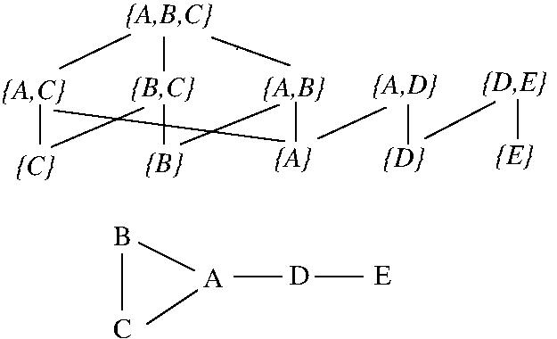
- EXAMPLE: The state space for the Maximum Clique
problem for a graph G.
The state space is the set of all subsets of vertices
of G that define clique-subgraphs, e.g., {A,B,C},
{D,E}, {E}. The neighbourhood of a state s is the
set of all states corresponding to those vertex-subsets
of G that induce clique-subgraphs and that can be
created by the addition or removal of a single vertex
to or from s, e.g., the neighbourhood of state {B,C}
is {{A}, {B}, {A,B,C}}.
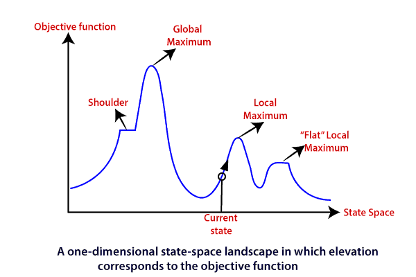
- These neighbourhoods, when combined with a
state-evaluation function, induce a state-space
landscape (Note that though the discussion and
algorithms below are phrased in terms of finding
maximum-value states on such landscapes, they can also
be rephrased in terms of finding minimum-value states,
e.g., (greedy) valley-descending search).
- EXAMPLE (RN3, Figure 4.1):
Useful features of such landscapes are:
- Global maximum: A state with the highest value
over all states in the state space.
- Local maximum: A state with the highest value
in that state's neighbourhood.
- Plateau: A set of adjacent states of the same value.
Can distinguish between local maximum plateau (all
states adjacent to the plateau have lower value
than the states in the plateau) and shoulder
plateau (some states adjacent to the plateau have
higher value than the states in the plateau).
Though global maxima are most desirable, local search
runs the (frequently unavoidable) risk of being trapped
in local maxima.
- Types of local search are distinguished by the methods
used to escape local maxima.
- Hill-climbing search (greedy search)
- This algorithm finds a local maximum, local
maximum plateau, or shoulder that is accesible
from the initial state.
- EXAMPLE: Basic hill-climbing search for
finding (maximal) cliques.
In what ways can hill-climbing search proceed
from state {A} in the graph above? State
{F}? State {E}? State {D1}?
- Not complete or optimal in general but is
typically fast and very memory-efficient.
- Is complete and optimal if the
state-space landscape has a particular
"dome" structure (Cormen et al
(2009), Section 16.4), e.g.,
Prim's and Kruskal's algorithms for
finding minimum spanning trees.
- Variants:
- Limited sideways-move hill climbing.
- Allows sideways moves in hopes that
an encountered plateau is actually a
shoulder.
- Need to limit the number of sideways
moves so you do not go into an
infinite loop on an actual plateau.
- Stochastic hill-climbing.
- Chooses at random among uphill moves
with uphill move probability
proportional to degree of solution
improvement.
- First-choice hill-climbing.
- Chooses at random among uphill moves
with uphill move probability
proportional to degree of solution
improvement until either a move resulting
in a state with a value better than
that of the current state is found or
there are no uphill moves from the
current state, i.e., a plateau has
been reached..
- Random-restart hill climbing.
- Implements common dictum: "If at
first you don't succeed, try again."
- Performs hill-climbing repeatedly
from randomly-chosen start states
until goal is found.
- Is complete, as one will eventually
generate the goal state.
- If probability of attaining a goal
from a randomly-chosen start state
is p, the expected number of
required restarts is 1/p.
- Though all of these variants are slower
than basic hill-climbing search, they
can be remarkably effective in certain
state-space landscapes, e.g. allowing up
to 100 sideways moves in a hill-climbing
search for the 8-Queens problem
increases the percentage of solved
instances from 14% to 94%.
- Local beam search
- Unlike hill-climbing, which only has one
current state, local beam search keeps track
of the best k states found so far and performs
hill-climbing simultaneously on all of them.
- EXAMPLE: Basic local beam search for
finding (maximal) cliques.
- Is not equivalent to running k independent
random-restart hill-climbing searches in
parallel; in local beam search, useful
information is passed between searches and
resources are focused dynamically where
progress is being made, i.e., "No progress
there? Help me over here!".
- Not complete or optimal in general but is
typically fast and very memory-efficient.
- Variants:
- Stochastic local beam search
- Chooses k new states at random among
uphill moves from the k current
states with uphill move probability
proportional to degree of solution
improvement.
- Analogous to natural selection in
biological evolution.
- Local search and its variants are characterized by an
increasing use of computer time as a substitute for
hand-crafted search strategy (Tony Middleton's "cook
until done") -- as such, these methods are a first
taste of the machine-crafted algorithms we will be
looking at in the final lectures of this course.
- Potential exam questions
Thursday, October 3 (Lecture #9)
[DC3200, Lecture #10;
RN3, Chapter 5; Class Notes]
Lines modified from the MaxValue (one-level) algorithm
are indicated by "<=".
ALGORITHM: MaxValue and MinValue (full tree)
1.   Function MaxValue(s)         Function MinValue(s)
2.     if leaf(s)                   if leaf(s)
3.       return eval(s)               return eval(s)
4.     v = -infinity               v = +infinity
5.     for (c in children(s))      for (c in children(s))
6.       v' = MinValue(c)            v' = MaxValue(s)
7.       if (v' > v) v = v'          if (v' < v) v = v'
8.     return v                    return v

     Initial Call: MaxValue(startState)
eval(s) returns score wrt the current (maximizing) player.
ALGORITHM: MaxValue and MinValue (limited-depth)
1.   Function MaxValue(s, d)     Function MinValue(s, d)       <=
2.     if (leaf(s) or d >= MaxD)    if (leaf(s) or d >= MaxD)    <=
3.       return eval(s)               return eval(s)
4.     v = -infinity               v = +infinity
5.     for (c in children(s))      for (c in children(s))
6.       v' = MinValue(c, d+1)       v' = MaxValue(c, d+1)     <=
7.       if (v' > v) v = v'          if (v' < v) v = v'
8.     return v                    return v

     Initial Call: MaxValue(startState, 0)
Lines modified from the MaxValue and MinValue (full tree)
algorithms are indicated by "<=".
ALGORITHM: MiniMax search (depth-limited)
1.   Function MiniMax(s, d, isMax)
2.     if (leaf(s) or d >= MaxD)
3.       return eval(s)
4.     if (isMax)
5.       v = -infinity
6.       for (c in children(s))
7.         v = max(v, MiniMax(c, d+1, false))
8.     else
9.       v = +infinity
10.      for (c in children(s))
11.        v = min(v, MiniMax(c, d+1, true))
12.    return v

       Initial call: MiniMax(startState, 0, true)
One final (and trivial) change is required to ensure
that the best action for the current (max) player to take is
stored in the start state.
ALGORITHM: MiniMax search (depth-limited) + saved best action [ASSIGNMENT #2]
1.   Function MiniMax(s, d, isMax)
2.     if (leaf(s) or d >= MaxD)
3.       return eval(s)
4.     if (isMax)
5.       v = -infinity
6.       for (c in children(s))
7.         v' = MiniMax(c, d+1, false)                       <=
8.         if (v' > v)                                       <=
9.           v = v'                                          <=
10.          if (d == 0) self.currentBestAction = c.action   <=
11.    else
12.      v = +infinity
13.      for (c in children(s))
14.        v = min(v, MiniMax(c, d+1, true))
15.    return v

       Initial call: MiniMax(startState, 0, true)
INTERLUDE: A look at the mechanics of
Assignment #2.
EXAMPLE: MiniMax generation and evaluation of an
altNim game tree from Assignment #2 (maxD = 2, i.e.,
two-move lookahead / startOdd = True / # given sticks = 6)
(see Test #3 in Assignment #2).
EXAMPLE: MiniMax generation and evaluation of an
altNim game tree from Assignment #2 (maxD = 3, i.e.,
three-move lookahead / startOdd = False / # given
sticks = 15) (see Test #6 in Assignment #2).
Potential exam questions
Tuesday, October 8
Thursday, October 10
- No lecture; class cancelled
Tuesday, October 15
- No lecture; midterm break
Thursday, October 17
- No lecture; class cancelled
Tuesday, October 22 (Lecture #10)
[DC3200, Lecture #10;
RN3, Chapters 5 and 6; Class Notes]
- Went over In-class exam # 1.
- Problem Solving and Search (Cont'd)
- Given that max(a, b) = -max(-a, -b), we can shorten the
MiniMax algorithm above to create the NegaMax algorithm.
- NegaMax is harder to understand and debug but it is the
version of MiniMax that is used in practice.
- ALGORITHM: NegaMax search (depth-limited)
1.   Function NegaMax(s, d, isMax)
2.     if (leaf(s) or d >= MaxD)
3.       return eval(s)
5.     v = -infinity
6.     for (c in children(s))
7.       v = max(v, -NegaMax(c, d+1, false))
12.    return v

       Initial call: NegaMax(startState, 0, true)
- Performance of MiniMax search
- MiniMax is complete wrt given maximum depth MaxD
- MiniMax is optimal wrt given maximum depth MaxD
- Time Complexity: O(b^{MaxD})
- Space Complexity: O(b * MaxD)
- MiniMax plays the Nash Equilibrium, i.e., each player
makes the best response to the possible actions of
the other player and thus neither player can gain by
deviating from the moves proposed by MiniMax.
- A closer examination of the intermediate results created
at the internal game tree nodes during MiniMax search
reveals that these results can be used to prune parts
of the game tree that cannot yield solutions better than
those that have been found so far.
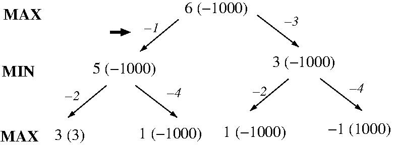
- EXAMPLE: MiniMax + pruning (one move each player)
[DC3200, Lecture #10, Slides 40-50
(PDF)]
- This optimization of MiniMax is known as AlphaBeta pruning.
- Introduces two new MiniMax parameters:
- alpha: Best alternative for the Max player on
this particular path through the game tree.
- beta: Best alternative for the Min player on
this particular path through the game tree.
- The interval [alpha, beta] is an ever-narowing window
as MiniMax search progresses which ``good'' paths
must pass through and thus allows other paths to be
pruned.
- ALGORITHM: MaxValue and MinValue (limited-depth + AlphaBeta)
1.   Function MaxValue(s, a, b, d)     Function MinValue(s, a, b, d)    <=
2.     if (leaf(s) or d >= MaxD)          if (leaf(s) or d >= MaxD)
3.       return eval(s)                    return eval(s)
4.     v = -infinity                     v = +infinity
5.     for (c in children(s))            for (c in children(s))
6.       v' = MinValue(c, a, b, d+1)       v' = MaxValue(c, a, b, d+1)  <=
7.       if (v' > v) v = v'                if (v' < v) v = v'
8.       if (v' >= b) return v             if (v' <= a) return v        <=
9.       if (v' > a) a = vi                if (v' < b) b = v'           <=
10.    return v                          return v

     Initial Call: MaxValue(startState, -infinity, +infinity, 0)
Lines modified from the MaxValue and MinValue (limited-depth)
algorithms are indicated by "<=".
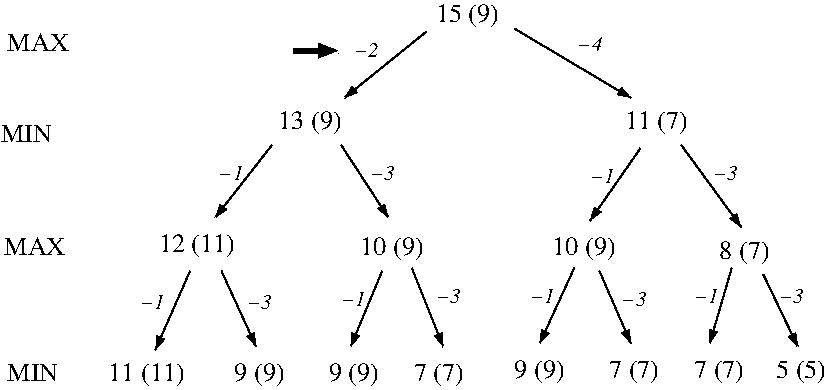
EXAMPLE: MaxValue + AlphaBeta pruning (two moves each player)
[DC3200, Lecture #10, Slides 56-110
(PDF)]
ALGORITHM: MiniMax search (depth-limited + AlphaBeta)
1.   Function MiniMax(s, a, b, d, isMax)                   <=
2.     if (leaf(s) or d >= MaxD)
3.       return eval(s)
4.     if (isMax)
5.       v = -infinity
6.       for (c in children(s))
7.         v' = max(v, MiniMax(c, a, b, d+1, false))       <=
8.         if (v' > v) v = v'                              <=
9.         if (v' > b) return v                            <=
10.        if (v' > a) a = v'                              <=
11.    else
12.      v = +infinity
13.      for (c in children(s))
14.        v' = min(v, MiniMax(c, a, b, d+1, true))        <=
15.        if (v' < v) v = v'                              <=
16.        if (v' <= a) return v                           <=
17.        if (v' < b) b = v'                              <=
18.    return v

       Initial call: MiniMax(startState, -infinity, +infinity, 0, true)
Lines modified from the MiniMax (limited-depth)
algorithm are indicated by "<=".
One final (and trivial) change is required to ensure
that the best action for the current (max) player to take is
stored in the start state.
ALGORITHM: MiniMax search (depth-limited + AlphaBeta + saved
best action)
1.   Function MiniMax(s, a, b, d, isMax)
2.     if (leaf(s) or d >= MaxD)
3.       return eval(s)
4.     if (isMax)
5.       v = -infinity
6.       for (c in children(s))
7.         v' = max(v, MiniMax(c, a, b, d+1, false))
8.         if (v' > v) v = v'
9.         if (v' > b) return v
10.        if (v' > a)                                       <=
11.          a = v                                           <=
12.          if (d == 0) self.currentBestAction = c.action   <=
13.    else
14.      v = +infinity
15.      for (c in children(s))
16.        v' = min(v, MiniMax(c, a, b, d+1, true))
17.        if (v' < v) v = v'
18.        if (v' <= a) return v
19.        if (v' < b) b = v'
20.    return v

       Initial call: MiniMax(startState, -infinity, +infinity, 0, true)
Lines modified from the MiniMax (limited-depth + AlphaBeta)
algorithm are indicated by "<=".
AlphaBeta pruning cuts the number of nodes searched by
MiniMax from O(b^d) to approximately 2b^{d/2} (which
can be proven to be the best possible). This allows
searches to depth d under MiniMax with a fixed amount
of computational resources to go to depth 2d under
MiniMax + AlphaBeta with the same resources, e.g.,
a previously bad gameplaying program can be enhanced to
beat a human world champion!
The MiniMax + AlphaBeta algorithm can be shortened
by rearranging the code above to be more
efficient; a runtime limit can also be enforced by
using the iterative deepening strrategy previously
applied to Depth-First Search in Lecture #5 (see
Lecture #10 of DC3200 for details).
Potential exam questions
- In most of our our previously discussed search algorithms
(cf. local search), our primary concern when solving
problems was more with sequences of actions that resulted
in goal states rather than the goal states themselves.
- Are there other types of search algorithms for problems
where the goal states are the primary concern?
- Let us focus on Constraint Satisfaction Problems
(CSPs).
- In a CSP, states have factored representations (see
Lecture #3) that are defined by a set of variables
X = {X1, X2, ..., Xn}, each of which has a value from
some variable-specific domain Di, and a set C of
constraints on the values of those variables.
- A constraint is described by a pair <(scope),
rel> where scope is a tuple of
variables from X and rel is a relation specifying
the values of the variables in rel allowed
by the constraint.
- The number or variables in scope determines
that constraint's arity (e.g., 1 = unary, 2 = binary,
3 = trinary, m = m-ary where m is arbitrary (global
constraint)).
- There are typically several ways to specify a
particular variable relation.
- EXAMPLE: We can specify the binary constraint on
variables X1 and X2 with common domain {A,B} that X1
and X2 have different values as <(X1,X2),[(A,B),(B,A)]>
or <(X1,X2), X1 \neq X2>.
- Each state in the state-space of a CSP specifies an
assignment of values [X1 = v1, X2 = v2, ..., Xn = vn]
to the variables in the CSP.
- A value-assignment that gives a value to each variable
in a CSP is said to be complete; if one or
more variables are not assigned values, the
value-assignment is partial.
- A value-assignment that satisfies all given constraints
in C for a CSP is said to be consistent; if one
or more constraints in C are not satisfed, the
value-assignment is inconsistent..
- A solution (goal state) for a CSP is a complete
consistent value-assignment for that CSP.
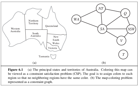
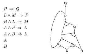
- EXAMPLE: A CSP for coloring a map of Australia.
- In map coloring, we want to assign colors to the
regions in the map such that no two adjacent regions
have the same color.
- Coloring a map of Australia (part (a)) can be modeled as
a CSP with variables X = {WA, NT, Q, NSW, V, SA, T}
over the common domain D = {red, green, blue} and
the binary constraints C = {SA \neq WA, SA \neq NT,
SA \neq Q, SA \neq NSW, SA \neq V, WA \neq NT, NT \neq
Q, Q \neq NSW, NSW \neq V} (where X \neq Y is
shorthand for the constraint <(X,Y) X \neq Y>)..
- Such a CSP with all binary constraints can be modeled
as a constraint graph (part (b)), which is an
undirected graph whose vertices correspond to variables
and edges correspond to constraints.
- CSPs with m-ary constraints, m >= 2, can be
modeled as constraint hypergraphs (See RN3,
Figure 6.2).
- There are many possible solutions for the map
coloring CSP above, e.g., [WA = red, NT = green,
Q = red, NSW = green, V = red, SA = blue, T = red].
- EXAMPLE: Soduku
- In soduku, one is a given a partial assignment from
the domain {1, 2, ..., 9} to the squares of a 9 x 9
grid (left) and we want to fill in the unassigned
squares such that no number appears twice in any
column, row, or 3 x 3 box (right).
- A CSP for a game of soduku corresponds to a set X of
81 variables (one for each square in the 9 x 9 grid)
over the common domain D = {1, 2, ..., 9}, a given
partial value-assignment to X wrt D (i.e., the
initially specified square-numbers), and a set C of
9 + 9 + 9 = 27 global constraints specifying that
the values of the 9 variables in each column, row,
and 3 x 3 box are different, e.g., AllDiff(A1, A2,
A3, A4, A5, A6, A7, A8, A9) for the first row in the
9 x 9 grid.
- One way of solving a CSP is to generate and evaluate all
possible value-assignments for that CSP's variables.
- This can be done in a tree with depth d = |X| and
branching factor b = max |Di|, where each level
assigns values to a particular variable and each leaf
encodes a complete assignment to the variables in X.
- This tree presupposes fixed orders on both the
variables on X and the values in each domain Di.
- EXAMPLE: A portion of a complete CSP value-assignment tree for
colouring a map of Australia:
- Generating complete value-assignment trees is
memory-expensive as such trees can have b^{d + 1} - 1 nodes;
can lower memory requirements by using Depth-First Search
to generate leaves one at a time.
- ALGORITHM: CSP DFS (RN3, Figure 6.5 variant)
1.   Function CSP_Search(csp)
2.     return CSP_DFS({}, 1, csp)

3.   Function CSP_DFS(assignment, d, csp)
4.     if (depth d = |X| + 1, i.e., assignment is complete, and
           assignment is consistent)
5.       return assignment
6.     else
7.       var = Xd
8.       for each value in Dd
9.         add {Xd = value} to assignment
10.        result = CSP_DFS(assignment, d + 1, csp)
11.        if (result \neq failure)
12.          return result
12.        remove {Xd = value} from assignment
13.    return failure
- The above fixes the memory problem but it is still
time-expensive as we may generate up to b^{d + 1} - 1 nodes
in the worst case.
Indeed, the NP-completeness of many CSP problems suggests
that such brute-force algorithms may be the best we can
do if we want to solve all input instances of such CSPs.
- ... But we typically don't want to solve all instances
of a particular CSP problem, only the ones we
encounter in practice -- can we do better in practice?
Thursday, October 24 (Lecture #11)
[RN3, Chapters 6 and 7; Class Notes]
- Problem Solving and Search (Cont'd)
- Constraint Satisfaction Problems (CSPs) (Cont'd)
- Let's start by unpacking the constraints from
leaf-evaluation.
- Observe that if a partial assignment does not satisfy
some constraint ci in C, no completion of this partial
assignment can satisfy ci. Hence,
we can stop search at any node whose partial assignment is
inconsistent with some constraint in C and thus prune the
subtree rooted at that node.
- ALGORITHM: CSP DFS + Partial (RN3, Figure 6.5 variant)
1.   Function CSP_Search(csp)
2.     return CSP_DFS2({}, 1, csp)

3.   Function CSP_DFS2(assignment, d, csp)
4.     if (depth d = |X| + 1, i.e., assignment is complete)    <=
5.       return assignment
6.     else
7.       var = Xd
8.       for each value in Dd
9.         if (value is consistent with assignment)          <=
10.          add {Xd = value} to assignment
11.          result = CSP_DFS2(assignment, d + 1, csp)
12.          if (result \neq failure)
13.            return result
14.          remove {Xd = value} from assignment
15.    return failure
Lines modified from the algorithm CSP DFS
are indicated by "<=".
- EXAMPLE: A portion of a CSP value-assignment tree for
colouring a map of Australia which allows pruning of
inconsistent partial assignment subtrees (dashed box):
- Further improvements arise from dynamic variable /
domain-value ordering heuristics.
- Variables can be ordered by the minimum-remaining
value (MRV) or degree heuristics, which
respectively prefer
the variables with the most constrained domains
and the variables that are involved in the largest
number of constraints, e.g., choose SA first in
coloring a map of Australia.
- Domain values can be ordered by the least-constraining
heuristic, which prefers values that rule out the
fewest choices for neighbouring values in the
constraint graph and thus allows maximum flexibility
for future value-choices.
- Good variable-ordering heuristics prune the largest
parts of search trees quickest (fail-first) while
good domain-value ordering heuristics consider first
those values most likely to lead to solutions
(fail-last).
- ALGORITHM: CSP DFS + Partial + Ordering (RN3, Figure 6.5 variant)
1.   Function CSP_Search(csp)
2.     return CSP_DFS3({}, csp)

3.   Function CSP_DFS3(assignment, csp)
4.     if (assignment is complete)
5.       return assignment
6.     else
7.       var = selectUnassignedVariable(csp, assignment)            <=
8.       for each value in orderDomainValues(var, assignment, csp)  <=
9.         if (value is consistent with assignment)
10.          add {var = value} to assignment
11.          result = CSP_DFS3(assignment, csp)
12.          if (result \neq failure)
13.            return result
14.          remove {var = value} from assignment
15.    return failure
Lines modified from the algorithm CSP DFS + Partial
are indicated by "<=".
- We can also make inferences over the constraints themselves
(constraint propagation) to
derive useful domain restrictions for variables.
- Such constraint consistency checks can involve one
or more constraints of varying constraint arities.
- Enforcing constraints that a variable has a
particular value (unary consistency),
e.g., the constraint <(SA) SA = red> that the SA
region of the map of Australia must be
colored red.
- Enforcing constraints on pairs of variables
(arc
consistency) such that every value in a
variable's domain can satisfy all binary
constraints containing that variable, e.g.,
the constraint <(WA,NT) WA \neq NT> is satisfied
by picking any color for WA and not picking the
same color for NT.
- Enforcing (sets of) constraints on 3 variables
(path consistency), e.g., WA, NT, and
SA are pairwise linked by difference constraints
and hence must have three different colors.
- Constraint propagation typically reduces the sizes
of variable domains; if in this process any variable
domain becomes empty, at least one of the type
of constraints being checked cannot be satisfied
by any assignment of values to the variables in the
CSP.
- ALGORITHM: AC-3 for arc consistency (RN3, Figure 6.3)
1.   Function AC-3(csp)
2.     q = queue({arcs in csp})
3.     while (q is not empty)
4.       (Xi, Xj) = q.pop()
5.       if revise(csp, Xi, Xj)
6.         if (|Di| = 0) return false
7.         for (each Xk \neq Xj that is a neighbour of Xi)
8.           q.add((Xk, Xi))
9.     return true

10.  Function revise(csp, Xi, Xj)
11.    revised = false
12.    for (each vi in Di)
13.      if (no value vj in Dj allows (vi,vj) to satisfy
              the constraint between Xi and Xj in csp)
14.        delete vi from Di
15.        revised - true
16.    return revised
- In the best case, constraint propagation derives solutions
and replaces search, e.g., constraint propagation algorithm
for map 2-coloring; however, it is more commonly done
as preprocessing for and subsequent interleaving with
search.
- ALGORITHM: CSP DFS + Partial + Ordering + Inference (RN3, Figure 6.5)
1.   Function CSP_Search(csp)
2.     return CSP_DFS4({}, csp)

3.   Function CSP_DFS4(assignment, csp)
4.     if (assignment is complete)
5.       return assignment
6.     else
7.       var = selectUnassignedVariable(csp, assignment)
8.       for each value in orderDomainValues(var, assignment, csp)
9.         if (value is consistent with assignment)
10.          add {var = value} to assignment
11.          inferences = getInferences(csp, var, assignment)       <=
12.          if (inferences \neq failure)                           <=
13.            add inferences to assignment                         <=
14.            result = CSP_DFS4(assignment, csp)
15.            if (result \neq failure)
16.              return result
1r.        remove {var = value} and inferences from assignment      <=
18.    return failure
Lines modified from the algorithm CSP DFS + Partial +
Ordering are indicated by "<=".
- More complex algorithm enhancements yield further
improvements in performance, e.g., intelligent
backtracking (backjumping).
- Local search may also be done with respect to CSPs, using
a state-space landscape based on complete assignments where
states are adjacent if they differ in a single variable
assignment and the state evaluation function is the number
of constraints in C that are not satisfied by the assignment
encoded in that state.
- ALGORITHM: MinConflicts (RN3, Figure 6.8)
1.   Function minConflicts(csp, maxSteps)
2.     current = an initial complete assignment for csp
3.     for i = 1 to maxsteps do
4.       if current is consistent return current
5.         var = a randomly-chosen conflicted variable from X
6.         value = the value v for var that minimizes
                    conflicts(var, v, current, csp)
7.         set var = v in current
8.     return failure

   conflicts(var, v, current, csp) returns the number of constraints
    in csp that would be violated by setting var to v in current
- Min-conflicts is surprisingly effective for many CSPs. For example,
the run-time of Min-conflicts on the n-Queens problem is
independent of problem size such that the million-Queens
problem is solved in an average of 50 steps!
Potential exam questions
Logical Reasoning
- Use richer representations of knowledge to go from
domain-specific search procedures to domain-general
search procedures. Here we will focus on knowledge
representations based on various logics.
- Knowledge-based agents
- knowledge base (KB) = set of (true) sentences.
- Interact with KB by TELL and ASK operations, both of
which may involve inference, i.e., creating new
sentences from old.
- Inference obeys the requirement that any new
sentences that are derived must follow
(in a technical sense we will discuss later) from
one or more of the sentences known from
previous TELL interactions or inferences.
- ALGORITHM: Knowledge-based agent percept->action computations (RN3, Figure 7.1)
1.   Function KB-Agent(KB, t, percept)
2.     TELL(KB, makePerceptSentence(percept, t))
3.     action = ASK(KB, makeActionQuery(t))
4.     TELL(KB, makeActionSentence(action, t))
5.     t = t + 1
6.     return action
- A KB initially encodes only background knowledge, and
is enriched both by percepts obtained during agent
interaction with the environment and inference over
that KB. As such, KB are often described at the
knowledge level, i.e., what is known and inferred,
rather than the implementation level, i.e., how what is
known is physically represented.
- An agent's behavior can be derived purely from a KB,
percepts, and inference (declarative approach) or
from hard-coded behaviors (procedural approach).
- Successful agents often combine these approaches,
using declarative knowledge for generality and
compiling this knowledge into procedural code when
necessary for efficiency.
EXAMPLE: Wumpus World (RN3, Figure 7.2)
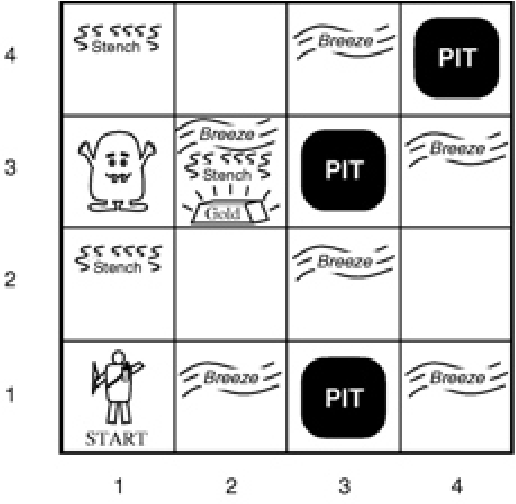
- Wumpus World (WW) is a puzzle game in which an agent
must explore a cave to find and return a cache of gold
while avoiding bottomless pits and the deadly wumpus.
- The WW problem is described as follows:
- Environment: A 4 x 4 square containing
one wumpus, one cache of gold, and several
bottomless pits. The agent always starts at
square [1,1] facing right and initially has no
knowledge of the environment except that agent's
percept at [1,1].
- Sensors: An agent has five one-bit sensors:
- Stench: Returns True if the wumpus (alive
or dead) is in same square as the agent or is
in a square directly (not diagonally)
adjacent to the agent.
- Breeze: Returns True if the agent is
directly adjacent to a bottomless pit.
- Glitter: Returns True if the agent
is in the same square as the cache of gold.
- Bump: Returns True if the agent walks
into one of the four walls surrounding the
grid.
- Scream: Returns True if the wumpus
dies after being struck by an arrow (see
below).
A percept will be given as a binary vector of the
current values for these sensors. For example, if
there is a stench and a breeze but no glitter,
bump or scream, the percept will be [S,B,-,-,-].
- Actuators: The agent can perform the
following actions:
- The agent can move forward one square
(Forward), turn left 90 o
(TurnLeft), or turn right 90 o
(TurnRight).
- If a move forward would cause an agent
to bump into a wall, the agent does
not move.
- If an agent enters a square with a live
wumpus or a bottomless pit, the agent
suffers a horrible death.
- The agent can Shoot its only arrow
forward in the direction the agent is facing.
- The arrow travels in that direction
until it either hits the wumpus (and
kills it) or strikes a wall.
- If the agent is in the same square as the
cache of gold, the agent can Grab the
cache.
- If the agent is on square [1,1], it can
Climb out of the cave.
- Performance Measure: +1000 for climbing out
of the cave with the gold, -1000 for falling into
a bottomless pit or being eaten by the wumpus,
-10 for shooting the arrow, and -1 for each other
action.
The game ends when the agent dies or climbs out of the
cave. Note that even if an agent lives, it may not be
successful, e.g., the cache of gold may be surrounded
by bottomless pits and hence inaccessible.
- The main challenge to an agent in WW is that agent's
initial ignorance of the configuration of the
environment; this ignorance is incrementally dispelled
by reasoning-guided exploration, e.g.,
- In [1,1], percept is [-,-,-,-,-]; squares [1,2]
and [2,1] are OK to move into => move to
square [2,1].
- In square [2,1], percept is [-,B,-,-,-]; squares
[2,2] and [3,1] may have bottomless pits =>
move back to [1,1] and then to [1,2].
- In [1,2], percept is [S,-,-,-,-]; the wumpus cannot
be in [2,2] (as stench would have been perceived
when visiting [2,1]) so the wumpus is in [1,3] and
[2,2] is OK => move to square [2,2].
- In [2,2], percept is [-,-,-,-,-]; squares [2,3] and
[3,2] are OK => move to square [2,3].
- In [2,3], percept is [S,B,G,-,-]; the cache of
gold is in this square => grab cache of gold,
retrace path to [1,1] on OK squares, and climb
out of the cave.
Several of the inferences made above, e.g., in (3), are
difficult because they involve knowledge gained at
different times and in different places.
- Note that when the agent draws a conclusion from
available information, that conclusion is only
guaranteed to be correct if the available information
is correct. Hence, it is critical that sensors
return correct values and actuators correctly
and completely perform requested actions.
Tuesday, October 29 (Lecture #12)
[RN3, Chapter 7; Class Notes]
- Logical reasoning (Cont'd)
- Logic: An Overview
- Each logic has an associated syntax and semantics, where
the syntax specifies all well-formed sentences in
that logic and the semantics specifies whether or
not each well-formed sentence in that logic is true with
respect to each possible world (or, more formally,
model).
- A possible world is a (potentially) real world
one or more agents exist within, while a model
is a mathematical abstraction which fixes the
truth or falsity of every relevant sentence
relative to variable-values proposed by that
model.
- If a sentence s is true in a model m, we say
that m satisfies s or m is a model of s.
- EXAMPLE: A possible world consists of x men and
y women sitting at a table playing bridge; as
a game of bridge requires exactly 4 players,
the sentence s = "x + y = 4" must be true.
Formally, all possible models for this world are
the assignments of non-negative
integers to x and y and the models that satisfy,
s are those that assign values to x and y that
add to 4, e.g., [x = 1 / y = 3], [x= 4 / y = 0].
- Given a definition of truth, we can now define logical
reasoning / inference as the process of correctly
deriving a conclusion s from a body of knowledge
KB (KB |-i s).
- a |= b means that sentence a entails sentence b,
i.e., b follows from a.
- More formally, a |= b if and only if M(a) \subseteq
M(b), i.e., in every model for which a is true, b
is also true.
- Given this definition of entailment, logical
inference is the process of deriving a valid
conclusion s from a knowledge base KB (sometimes
written as KB |-i s).
- Think of all consequences of KB as a haystack and
a particular consequence s as a needle.
Entailment can say whether or not a specified
needle is in a haystack, and inference is the
finding of that needle.
- Model checking is an inference procedure that
enumerates all possible worlds and for a sentence
s checks if s is true in all models for which KB
is true; as such, it shows one way in which
entailment can be used to derive conclusions.
- EXAMPLE: Model checking for Wumpus World (RN3, Figure 7.5)
- Let KB be the KB at the beginning of step (2) in
the reasoning-based exploration of WW above.
Relative to KB, consider the following two
sentences:
- a1 = "There is no pit in [1,2]".
- a2 = "There is no pit in [2,2]".
- From inspection, we can see that for every model
in which KB is true, a1 is also true and hence
KB |= a1. However, we can also see that in some
models in which KB is true, a2 is false, i.e.,
KB |\= a2. Hence we can conclude that there is
a no pit in [1,2] but we cannot conclude that
there is not (or, for that matter, is) a pit
in [2,2].
- Desirable properties of inference algorithms:
- Soundness (Truth-preserving); An inference algorithm
that only derives entailed conclusions is
sound, i.e., the inference
algorithm does not make up things.
- Completeness: An inference procedure that can derive
any conclusion that is entailed is complete,
i.e., it is not the case that there are entailed
conclusions that the inference algorithm
cannot derive.
- Logical reasoning should also be grounded in the
real world, i.e., if s is derived from a KB by a
sound inference procedure then s should be true in the
real world. One does this by making sure sensors and
actuators are correct (grounded percepts) and taking
care in grounding inference rules in the real world.
- Propositional logic (PL)
- Syntax
- Sentences in PL can be atomic sentences consisting of a
single Boolean literal, i.e., True, False, or
propositional symbol, e.g., P, Q, R, or complex
sentences built up using logical connectives, e.g.,
not, and, or, => (implies), <=> (if and only if), and
parentheses.
- Though there is a precedence order on logical
connectives, it is perhaps best to use
parentheses to denote the wanted recursive
structure of complex sentences.
- Syntax of PL (RN3, Figure 7.7)
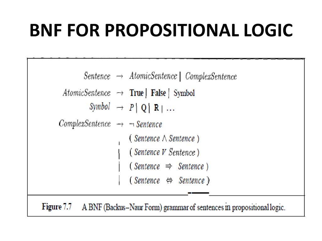
- Semantics
- The truth value of a sentence s in PL for a given
model M is built up recursively in a bottom-up
fashion from the truth-values of the propositional
symbols in s wrt M by applying the truth tables for
the logical connectives in s, e.g.,
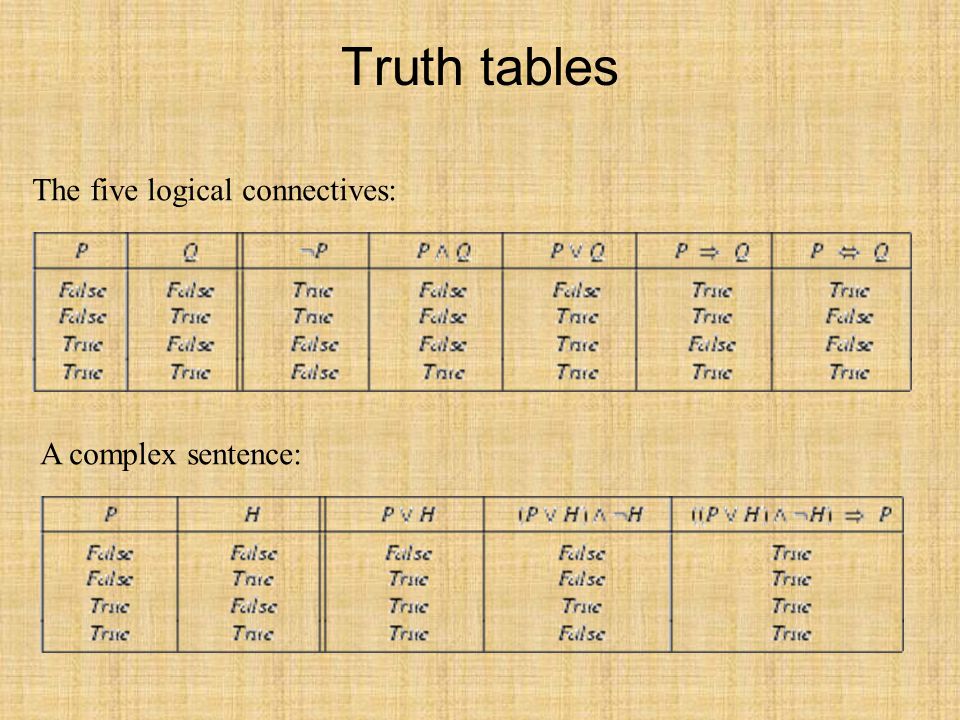
The truth table for => is
counterintuitive because P => Q (unlike
natural language "if P then Q") does not imply causation
or relevance between P and Q, e.g., "5 is odd => Tokyo
is the capital of Japan" is true in PL. Rather, P => Q
should be interpreted as "If P is true then I am claiming
Q is true; otherwise, I am making no claim".
- EXAMPLE: A PL KB for Wumpus World
- Focus for now on the immutable aspects of WW.
This will be done for each location [x,y] in the
cave with the following symbols:
- Pxy: True if there is a pit in [x,y].
- Wxy: True if there is a wumpus (dead or
alive) in [x,y].
- Bxy: True if the agent perceives a breeze in
[x,y].
- Sxy: True if the agent perceives a stench in
[x,y].
- The following sentences will suffice to derive
not P12 (there is no pit in [1,2]):
- R1: not P11 (there is no pit in [1,1])
- R2: B11 <=> (P12 or P21)
- R3: B21 <=> (P11 or P22 or P31)
- R4: not B11
- R5: B12
- PL Inference procedures
- Given a knowledge base KB and a sentence s in in
PL, we want to determine if KB |= s, e,g,
for the WW KB, is it the case that KB |= not P12?
- We will here consider two broad classes of
inference procedures: model checking and theorem
proving.
- Model checking
- Advanced model checking
- We will look at two families of
algorithms that perform well in practice
using model-tree pruning and local
search, respectively.
- We also i) rephrase entailment statements
KB => s {which is equal to not KB or s)
as determining the unsatisfiability of
(KB and not s) (which is obtained from
the above by applying DeMorgan's Law)
and ii) rephrase both KB and s in
Conjunctive Normal Form (CNF) in
which a sentence is a conjunction (AND)
of disjunctive (OR) clauses, e.g.,
(A or not
B) and (B or not C or D) and (B or D).
- There is a standard procedure for
transforming an arbitrary PL
sentence into a CNF equivalent
(RN3, pp. 253-254).
- As many other problems can be reduced
to CNF SAT, our derived algorithms
have a much broader applicability.
- Backtracking + heuristics
(Davis-Putnam-Logeman-Loveland (DPLL))
- DPLL is a depth-first search of
the model-tree that uses partial
model unsatisfiability and
various sentence-reducing
heuristics to prune subtrees
containing non-satisfying
models, e.g.,
- Pure heuristic: Assign pure
symbols (symbols that have
the same sign in all
occurrences) the value that
makes them true.
- Unit heuristic: Assign symbols
in single-symbol clauses the
value that makes them true.
Note that both heuristics when
invoked may trigger a cascade
of subsequent sentence reductions.
- ALGORITHM: DPLL-Satisfiable?
(RN3, Figure 7.17)
1.   Function DPLL-Satisfiable?(s)
2.     sym = list of proposition symbols in s
3.     cls = list of clauses in CNF representation of s
4.     return DPLL(cls, sym, {})

5.   Function DPLL(cls, sym, model)
6.     if every clause in cls is true in model return true
7.     if some clause in cls is false in model return false
8.     (P, value) = Find-Pure-Symbol(sym, cls, model)
9.     if P is non-null return DPLL(cls, sym - P, model + {P = value})
10.    (P, value) = Find-Unit-Clause(cls, model)
11.    if P is non-null return DPLL(cls, sym - P, model + {P = value})
12.    P = First(sym)
13.    rest = Rest(sym)
14.    return (DPLL(cls, rest, model + {P = true}) or
               DPLL(cls, rest, model + {P = false}))
- A variety of scale-up enhancements
to the DPLL algorithm, e.g.,
variable and value ordering, allow
modern SAT solvers to tackle
input instances with tens of
millions of variables.
- Local search
- Uses a model-evaluation function
h(m) that counts the number of
clauses in the given instance of
CNF SAT that are not satisfied
by m.
- At each step, the algorithm picks
an unsatisfied clauses and
selects at random one of two
ways to chose a variable in that
clause to flip.
- ALGORITHM: WalkSAT (RN3, Figure 7.18)
1.   Function WalkSAT(cls, p, maxFlips)
2.     model = random assignment of true / false to symbols in cls
3.     for i = 1 to maxFlips do
4.       if model satisfied all clauses in cls return model
5.       c = randomly-selected clause in cls that is false in model
6.       with probability p
7.         flip the value in model of a randomly-selected
            symbol in cls
8.       else
9.         flip the value in model of whichever symbol in cls whose
             flipped value maximizes the number of satisfied clauses
10.    return failure
- A returned failure can mean either
that we did not give the algorithm
enough time or that the given
sentence is unsatisfiable; only
the former can be fixed by
increasing maxFlips. Hence,
WalkSAT is more commonly used when
we expect that a solution exists
then when we need to show
unsatisfiability / entailment.
Wednesday, October 30
Thursday, October 31 (Lecture #13)
[RN3, Chapter 7; Class Notes]
This rule is sound (RN3, p. 253).
Observe that if repeated applications
of the resolution rule to a CNF
sentence s results in the empty clause
then s is unsatisfiable (as a
disjunctive clause is true if and only
if that clause has at least one literal
that evaluates to true). Given that
KB |= s if and only if (KB and not s)
is unsatisfiable, we now have a
resolution-based algorithm for proving
entailment.
EXAMPLE: Theorem Proving by Hand in
Wumpus World (Part III)
- Suppose the agent in WW is in [1,1], perceives
no breeze, and wishes to establish that there is
no pit in [1,2], i.e., not P12. The relevant
knowledge base is
KB = R2 and R4 = (B11 <=> P12 or P21) and not B11
which means that
KB and not (not P12)= ((B11 <=> P12 or P21)
and not B11 and P12)
whose CNF form has five disjunctive clauses:
- C1: not P21 or B11
- C2: not B11 or P12 or P21
- C3: not P12 or B11
- C4: not B11
- C5: P12
Observe that the resolution of C3 and C4 gives
clause (not P12), whose resolution with C5 is the
empty clause. Hence, there is no pit in [1,2].
ALGORITHM: PL-Resolution (RN3,
Figure 7.12)
1.   Function PL-Resolution(KB, s)
2.     cls = list of clauses in CNF representation of (KB and not s)
3.     new = {}
4.     while (true)
5.       for each pair of clauses (ci, cj) in cls do
6.         resolvents = PL-Resolve(ci, cj)
7.         if resolvents contains the empty clause return true
8.         new = new + resolvents
9.       if new \subseteq cls return false
10.      cls = cls + new

      PL-Resolve(c1, c2) returns the set of all possible clauses
       obtained by resolving c1 and c2.
It can be shown that this algorithm is
both sound (RN3, p. 253) and complete
(RN3, pp. 255-256).
There are a number of cases in which the
full power of resolution is not needed
to do logical inference. One restricted case
that allows efficient (indeed, linear time)
inference is knowledge bases composed of
definite clauses.
- A definite clause is a disjunction of
one or more literals in which exactly
one literal is positive, e.g., (not P or
Q), (P or not Q or not R), and (R) are
all definite clauses while (not P or
not R) and (not Q) are not.
- Knowledge bases containing only definite
clauses are interesting for three
reasons:
- Any definite clause can be
rewritten as a conjunction of the
negations of the negated literals
(the clause's premise) that
implies the unnegated literal
(the clauses' conclusion),
e.g., (P or not Q or not R)
is logically equivalent to
(Q and R) => P. A definite
clause with one literal is
logically equivalent to True and
is called a fact.
- Logical inference over definite
clauses can be done by either
the forward or backward chaining
algorithms.
- Both of these algorithms, when
implemented carefully, run in
time linear in the size of KB.
- Both of these algorithms can perhaps
best be explained by visualizing
a definite clause KB as an AND-OR
graph.
- An AND-OR graph is a directed
graph in which each non-leaf
vertex is either an AND vertex
or an OR vertex.
- A definite clause KB can converted
to an AND graph in which:
- each symbol is a vertex;
- each fact is a leaf;
- each symbol which is the
conclusion of exactly one
clause is an AND-vertex
which is connected to the
symbol-vertices in that
clause's premise; and
- each symbol which is the
conclusion of multiple clauses
is an OR-vertex connected to
the AND-vertices
corresponding to these
clauses, each of which
is in turn connected to the
symbol-vertices in their
respective premises.
- EXAMPLE: A definite clause KB and its
associated AND-OR graph (RN3,
Figure 7.16)
In the examples below, the five clauses
will be abbreviated as Q, P, M, L1, and
L2, respectively.
Tuesday, November 5 (Lecture #14)
[RN3, Chapter 7; Class Notes]
- Logical reasoning (Cont'd)
- Propositional logic (PL) (Cont'd)
The facts required for BC to
derive each possible implication
relative to these clauses
are given in the following table:
| Derivable implications |
Required Facts |
| A |
B |
C |
D |
| S1 |
X |
X |
|
|
| S2 |
X |
|
X |
X |
| S3 |
|
|
X |
X |
| D1 |
X |
X |
X |
X |
| D2 |
X |
|
X |
X |
Note that we are assuming here that each
implication can only be derived in one
way and hence has only one set of
required facts. If an implication was
derivable in several ways, we would have
to list for each implication the
fact-sets relative to which that
implication would be derived. For
example, if there was an additional
clause "B + C => S1" in the above,
S1 would be derivable via the fact-sets
{A,B} and {B,C}.
- BC as given here can state whether
or not the available facts allow
a proof of a specified implication;
however, it does not give any let
alone all such proofs (which is
required for explainability, e.g.,
medical diagnosis).
INTERLUDE: A look at the mechanics of
Assignment #3.
Potential exam questions
Thursday, November 7
Tuesday, November 12 (Lecture #15)
[RN3, Chapter 7; Class Notes]
Potential exam questions
Thursday, November 14 (Lecture #16)
[DC3200, Lecture #12;
Class Notes]
Potential exam questions
Tuesday, November 19 (Lecture #17)
[DC3200, Lecture #14;
RN3, Chapter 21; Class Notes]
- Reinforcement Learning (RL)
- Reinforcement learning is a type of machine learning that is
inspired by mechanisms in Behavioral psychology.
- RL proposes learning through interactions with an
environment where each action has an associated
positive or negative reward, e.g., pleasure or pain.
- There is no explicit teacher, e.g., the
training set of correct (input-output) examples
in supervised learning; rather, teaching is both
implicit in and localized to action rewards.
- There is no evolution of a population as in EC but
rather updating over time of an individual's
beliefs about situation-appropriate actions
in response to interactions with an environment.
- The goal of an RL agent is to maximize summed rewards
over time.
- RL can implement problem-solving by structuring the
environment and action rewards to achieve a goal,
e.g., structuring a human community to enforce a
utopia (Skinner (1948)).
- RL is not an algorithm but rather a problem specification
method -- there are many algorithmic techniques for
solving RL-specified problems.
- The overall structure of reinforcement learning:
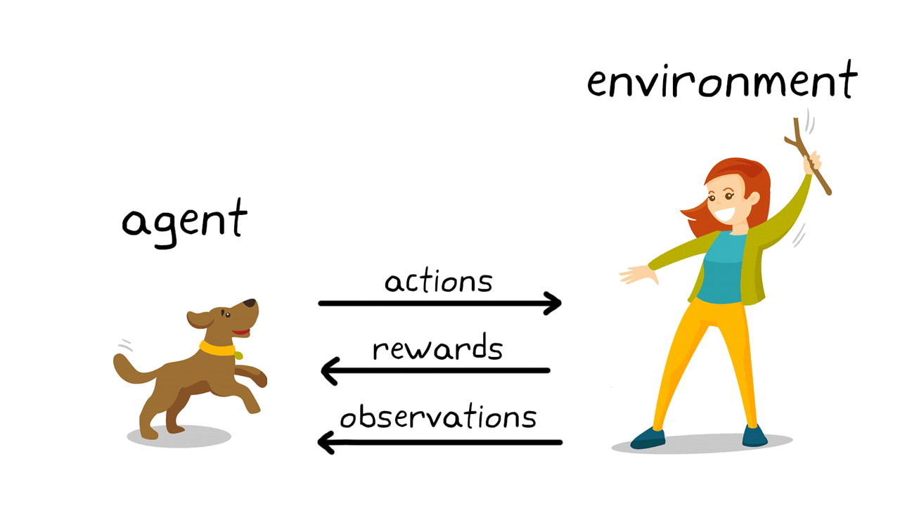
- The reinforcement learning loop:
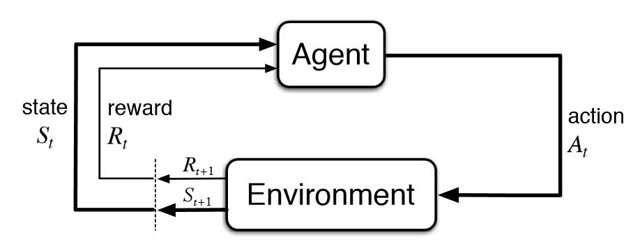
- EXAMPLE: The Cart-Pole and Mountain Car problems as
formulated in RL {DC3200 Lecture #14, Slides 19-21
(PDF)]
- The four components of an RL-specified problem:
- Agent
- Environment
- Policy
- A policy is a mapping from states of the environment
to the actions to be taken at those states.
- A policy is the core component of an RL agent in
that it defines that agent's behavior.
- Can be implemented by a variety of deterministic or
stochastic mechanisms, e.g., lookup table (see
Lecture #2), finite-state machine, neural network.
- EXAMPLE: Blackjack tabular policy [DC3200 Lecture
#14, Slide #26 (PDF)]
- Policies change over time in response to
interactions as specified by the chosen RL
algorithm.
- Reward function
- Maps each perceived state (or state-action
pair) to a single number (the reward); as
such, it implicitly defines the goal of an
RL-specified problem.
- Rewards come from the environment, not the agent.
- The agent's goal is to maximize the expected
summed rewards over time (that agent's
return).
- EXAMPLE: Reward function for finding a
shortest path.
- Goal is terminal state (the destination).
- Non-goal states have reward -1.
- Getting to goal in the fewest number of steps
maximizes the summed rewards / return.
- EXAMPLE: Reward function for learning to bet
well on horse races.
- Winning bet = positive reward proportional to
money won.
- Losing bet = negative reward proportional to
money lost.
- Learning to bet well maximizes the summed
rewards / return over time.
- An optimal policy maximizes the expected return
over time; how can we quantify expected return?
=> value functions!
- If a reward function tells us what is immediately
good, a value function indicates what is
expected (in the probabilistic sense) to
eventually be good or bad over time, i.e.,
long-term good.
- The value of a state s or state-action-pair
(s,a) is the return an agent can expect to
accumulate in the future given that it is
currently in s or currently in s and performs
action a.
- Value is much harder to determine than rewards,
and requires more complex calculation and
estimation techniques.
- EXAMPLE: Value function for finding a
shortest path.
- Let non-goal states have values inversely
proportional to the lengths of the shortest
path from those states to the goal.
- Actions which take us to high-value states have
the highest value.
- EXAMPLE: Value function for learning to bet
well on horse races.
- Let individual horses have bet-values
proportional
to their records of winning past races.
- Horses with the best records of winning past
races have the highest probability of winning
the current race (as well as future races)
and hence bets on such
horses have the highest value.
- An agent's policy should ideally prefer at each
possible state not the highest-reward action but
rather the highest-value action.
- One of the main challenges in RL is the trade-off between
exploration and exploitation.
- To maximize rewards, an agent must prefer actions that
it knows produce good results, i.e., the agent must
exploit knowledge it has.
- In order to learn which actions produce good results,
an agent must first try a wide range of actions, i.e.,
the agent must explore to acquire knowledge.
- This is also frequently a challenge in real life.
- EXAMPLE: When choosing a restaurant, do you eat at
somewhere you've had a good meal in the past or try
somewhere new?
- EXAMPLE: When betting on horse races, do you bet on a
horse that won for you before or bet on a new horse?
- There are a wide variety of algorithmic techniques for
implementing RL and dealing with the issues mentioned
above, e.g., Temporal Difference Learning, Monte Carlo RL,
Q-Learning; please see Sutton and Barto (2018) (a truly
excellent textbook, available online for free to boot)
and Chapter 21 of RN3 for details.
- Potential exam questions
Thursday, November 21 (Lecture #18)
[DC3200 Lecture #19 and
Lecture #20;
RN4, Chapter 21; Class Notes]
Friday, November 22
Tuesday, November 26
- Guest Lecture: Data Representations as a Driving Force in
AI Research
(Dr. Rory Campbell, University of Western Ontario)[PDF]
Thursday, November 28 (Lecture #19)
[Class Notes]
- Epilogue: The Future of Algorithmic Methods for AI
References
- Adolfi, F., Vilas, M., and Wareham, T. (2024a) "`Complexity-Theoretic
Limits on the Promises of Artificial Neural Network
Reverse-Engineering." In the Proceedings of the 46th Annual Meeting
of the Cognitive Science Society (CogSci 2024).
- Adolfi, F., Vilas, M., and Wareham, T. (2024b) "The Computational
Complexity of Circuit Discovery for Inner Interpretability."
arXiv.2410.08025 (71 pages).
[PDF]
- Barcelo, P., Monet, M., Perez, J., and Subercaseaux, B. (2020) "Model
interpretability through the lens of computational complexity." In
Advances in neural information processing systems, 33, 15487-15498.
[PDF]
- Bassan, S., Amir, G., and Katz, G. (2024) "Local vs. Global
Interpretability: A Computational Complexity Perspective."
arXiv preprint arXiv:2406.02981.
[PDF]
- Bellogín, A., Grau, O., Larsson, S., Schimpf, G., Sengupta, B., and
Solmaz, G. (2024) "The EU AI Act and the Wager on Trustworthy AI."
Communications of the ACM, 67(12), 58-65.
[PDF]
- Buyl, M. and De Bie, T. (2024) "Inherent Limitations of AI Fairness."
Communications of the ACM, 67(2), 48-55. [HTML]
- Bylander, T. (1994) "The Computational Complexity of Propositional
STRIPS Planning.: Artificial Intelligence, 69(1-2), 165-204.
- Cormen, T.H., Leiserson, C.E., Rivest, R.L., Stein, C. (2009)
Introduction to Algorithms. Third Edition. The MIT Press;
Cambridge, MA. [Abbreviated above as CLRS]
- Dhar, V. (2024) "The Paradigm Shifts in Artificial Intelligence."
Communications of the ACM, 67(11), 50-59. [HTML]
- Fikes, R.E. and Nilsson, N.J. (1971) "STRIPS: A New Approach to the
Application of Theorem Proving to Problem Solving." Artificial
Intelligence, 2(3-4), 189-208.
- Garey, M.R. and Johnson, D.S. (1979) Computers and
Intractability: A Guide to the Theory of NP-Completeness.
W.H. Freeman; San Francisco, CA.
- Guest, O. and Martin, A. E. (2023) "On logical inference over brains,
behaviour, and artificial neural networks." Computational Brain &
Behavior, 6(2), 213-227
[PDF]
- Guest, O. and Martin, A.E. (2024) "A Metatheory of Classical and
Modern Connectionism." Preprint. [PDF]
- Haigh, T. (2023a) "Conjoined Twins: Artificial Intelligence and the
Invention of Computer Science." Communications of the ACM,
66(6), 33-37. [HTML]
- Haigh, T. (2023b) "There was No 'First' AI Winter." Communications
of the ACM, 66(12), 35-39. [HTML]
- Haigh, T. (2024a) "How the AI Boom Went Bust." Communications
of the ACM, 67(2), 22-26. [HTML]
- Haigh, T. (2024b) "Between the Booms: AI in Winter." Communications
of the ACM, 67(11), 19-23. [HTML]
- Haigh, T. (2025) "Artificial Intelligence: Then and Now." Communications
of the ACM, 68(2), 24-29. [HTML]
- Huxley, J. (1957) New Bottles for New Wine. Chatto & Windus.
- Kedia, A, and Rasu, M. (2020) Hands-On Python Natural Language
Processing. Packt Publishing; Birmingham, UK.
- Livni, R., Shalev-Shwartz, S., and Shamir, O. (2014) "On the
computational efficiency of training neural networks." Advances
in Neural Information Processing Systems, 27, 1-9.
- Marcus, G. and Davis, E. (2019) Rebooting AI: Building Artificial
Intelligence We Can Trust. Pantheon Books; New York.
- Marcus, G. and Davis, E. (2021) "Insights for AI from the Human Mind",
Communications of the ACM, 64(1), 38-41. [Text]
- Newell, A. and Simon, H.A. (1956) The Logic Theory Machine: A
Complex Information Processing System. RAND Technical
Report P-868.
- Newell, A., Shaw, J.C., and Simon, H.A. (1959) Report on a General
Problem Solving Program. RAND Technical Report P-1584.
- Newell, A. and Simon, H.A. (1972) Human Problem Solving.
Prentice-Hall.
- Russell, S. and Norvig (2010) Artificial Intelligence: A Modern
Approach (3rd Edition). Prentice-Hall.
- Russell, S. and Norvig (2022) Artificial Intelligence: A Modern
Approach (4rd Edition). Prentice-Hall.
- Schmidhuber, J. (2015) "Deep learning in neural networks: An
overview." Neural Networks, 61, 85-117.
- Seuss, Dr. (1970) One fish two fish red fish blue fish.
Random House.
- Shein, E. (2024) "The Impact of AI on Computer Science Education."
Communications of the ACM, 67(11), 13-15.
[HTML]
- Skinner, B.F. (1948) Walden Two. Hackett Publishing
Company.
- Song, L., Vempala, S., Wilmes, J., and Xie, B. (2017) "On the
complexity of learning neural networks." In Advances in Neural
Information Processing Systems, 30, 1-9.
- Sutton, R.S. and Barto, A.G. (2018) Reinforcement Learning: An
Introduction (Second Edition). The MIT Press.
[Website]
- Van Rooij, I., Guest, O., Adolfi, F., de Haan, R., Kolokolova, A.,
and Rich, P. (2024) "Reclaiming AI as a theoretical tool for
cognitive science." Computational Brain & Behavior, 1-21.
[PDF]
- Wareham, T. (2022) "Creating Teams of Simple Agents for Specified
Tasks: A Computational Complexity Perspective."
CoRR abs/2205.02061 (20 pages).
[PDF]
- Wareham, T. and Vardy, A. (2018) "Putting It Together: The
Computational Complexity of Designing Robot Controllers and
Environments for Distributed Construction." Swarm
Intelligence, 12(2), 111-128.
Created: June 26, 2024
Last Modified: January 23, 2025