Computer Science 6901, Fall '26
Course Diary

---

Copyright 2026 by H.T. Wareham
All rights reserved

---

Week 1, Week 2, Week 3, (In-class Exam #1 Notes),
Week 4. Week 5, (end of diary)

Thursday, September 10 (Lecture #1)
[Sections 1.1-1.2]

• Introduction to course; dates and conventions.
• Interlude: Why do a course like this in 2026?
  • Algorithms and their analysis and design has traditionally been seen as central to Computer Science. Such analysis and design typically encompasses four activities:
    1. Figure out exactly what problem needs to be solved (including all relevant restrictions that may hold relative to your particular instance of this problem).
    2. Determine if an efficient algorithm for your problem in (1) relative to its relevant restrictions already exists. If there is a range of possible algorithms, pick the best one.
    3. If you can't find an existing efficient algorithm in (2), design one using existing techniques, e.g., combinatorial solution-space trees, divide and conquer, dynamic programming, greedy algorithms, exploiting advanced data structures.
    4. If you cannot design an efficient algorithm in (3), apply computational complexity analysis to see if efficient algorithms for your problem are impossible; if so, see what alternatives exist, e.g., randomized algorithms, cost-approximation algorithms, parameterized algorithms, heuristics, and pick the best one.

  • Some claim that, given AI's new-found abilities to automate writing computer programs, AI can also do algorithm design and analysis. While AI can help with some of the activities above, it cannot do all of them as well as a human being yet (and maybe even ever)
  • Example: Asking Gemini for the most efficient algorithms for finding shortest paths in cities.
  • Given this, humans are for now still very much necessary to algorithm design and analysis, and you as CS students should do at least one course like this.
• Background: Problems and Algorithms
  • Computational Problems
    • A computational problem is a relation between inputs and outputs.
    • Types of computational problems.
      • By type of output:
        • Decision problem: Returns a Boolean value (typically the answer to a question about the optimal solution for a given instance of a problem).
        • Cost / Evaluation problem: Returns a number (typically the cost of an optimal solution for a given instance of a problem).
        • Example / Solution problem: Returns a structure (typically an optimal solution for a given instance of a problem).
        • Example: Versions of the Shortest Path problem:

          Shortest Path (Unweighted) [Decision]
          Input: A graph G = (V,E), two vertices u and v in V, and a positive integer k.
          Question: Is there a path P in G from u to v such that the number of edges in P is <= k?

          Shortest Path (Unweighted) [Evaluation]
          Input: A graph G = (V,E) and two vertices u and v in V.
          Output: The length of the path in G from u to v with the smallest possible number of edges.

          Shortest Path (Unweighted) [Solution]
          Input: A graph G = (V,E) and two vertices u and v in V.
          Output: A path P in G from u to v such that the number of edges in P is the smallest possible.

      • By entities in I/O relation:
        • Discrete problem: Manipulates integers and/or discrete structures.
        • Numerical problem: Manipulates (arbitrary-precision) real numbers in addition to integers and/or discrete structures.
    • This course will focus on various discrete problems. In particular, we will be looking at a number of discrete problems in which we are looking for a substructure of a given structure that is optimal relative to some function (combinatorial optimization problems).
    • Guidelines for defining computational problems
      • Strike balance between abstraction, formalization, and phrasing in terms of stated entities -- the former exposes the mathematical structures underlying a problem, the latter keeps the problem relevant.
      • Abstraction useful as it may show that your problem is the same as one that has already been solved
        => The first rule of algorithm design is don't <=

      • Make sure that the problem you defined and subsequently will be working on is the one you actually need to solve, e.g., checking possibility of vs checking costs of vs checking routes for airline flights.
    • Example: Bob's Trucking Company.
      • Examine contents of all depots in a shipping network => graph traversal (assuming shipping network can be modeled as a graph in which vertices are depots and edges are routes).
      • Minimizing costs associated with deliveries => shortest paths (# edges / summed edge-lengths)

        Shortest Path (Unweighted)
        Input: A graph G = (V,E) and two vertices u and v in V.
        Output: A path P in G from u to v such that the number of edges in P is the smallest possible.

        Shortest Path (Weighted)
        Input: An edge-weighted graph G = (V,E,W) and two vertices u and v in V.
        Output: A path P in G from u to v such that the sum of the weights of the edges in P is the smallest possible.

      • Maximizing reimbursements associated with deliveries => longest paths (# edges / summed edge-lengths)

        Longest Path (Unweighted)
        Input: A graph G = (V,E) and two vertices u and v in V.
        Output: A path P in G from u to v such that the number of edges in P is the largest possible.

        Longest Path (Weighted)
        Input: An edge-weighted graph G = (V,E,W) and two vertices u and v in V.
        Output: A path P in G from u to v such that the sum of the weights of the edges in P is the largest possible.

      • Maximizing the value of items loaded on a truck with a specified maximum capacity, where truck must carry all or none of each item => 0/1 Knapsack
        0/1 Knapsack
        Input: A set U of items, an item-size function s(), an item-value function v(), and a positive integer B.
        Output: A subset U' of U such that the sum of the sizes of the items in U' is less than or equal to B and the sum of the values of the items in U' is the largest possible.

      • Minimizing the number of emergency aid depots required in a shipping network such that at least one of the endpoints of each route has such a depot => Vertex Cover

        Vertex Cover
        Input: An undirected graph G = (V,E).
        Output: A subset V' \subseteq V such that for all edges (u,v) \in E, at least one of u and v is in V', and the size of V' is the smallest possible.

  • Algorithms
    • An algorithm for a problem is a finite sequence of instructions relative to a particular computer-model that, given an input for that problem, computes the corresponding output.
      • This is the classicial definition of an algorithm.
      • Such algorithms are hand-crafted by human beings and are not the same as procedures developed by computational methods (e.g., backpropogation, reinforcement learning) that are encoded in particular devices (e.g., neural networks), e.g. social media content choice algorithms, ChatGPT.
    • Types of algorithms.
      • By mode of algorithm creation: hand-crafted vs machine-crafted.
      • By type of computer-model:
        • Instruction execution mode: Deterministic / Randomized / Nondeterministic
        • Number of processors: Serial (single processor) / Parallel (multiple processors)
      • By type of computation: Discrete / Numerical.
    • This course will focus on hand-crafted deterministic serial discrete algorithms.
  • There are typically many possible algorithms for a particular problem. Which algorithm should we use? Perhaps we should use the one that is most efficient -- this, however, requires a useful and usable measure of algorithm efficiency ... This will be the topic of our next lecture.
• Potential exam questions

Tuesday, September 15 (Lecture #2)
[Sections 2.1-2.2 and 3.1]

• Background: Time Complexity
  • Algorithms as technology: Algorithms are at least as (and sometimes more) important to efficient computing than traditional electronic technologies like microprocessors and memory chips (Jim Dawe's Bonus, Need's Video Sorting).
  • Desirable properties of a measure of algorithm efficiency:
    • Machine independent.
    • Function of input size.
    • Useful for both assessing individual and comparing groups of algorithms.
    • Mathematically tractable, i.e., can be derived (relatively) easily for any algorithm.
  • For most of this course, we will focus on efficiency wrt algorithm running time; however, we will occasionally mention other measures, i.e., space (computer memory).
  • The road from actual running time to asymptotic worst-case time complexity -- necessary lies (or rather, abstractions):

    		C(x)		T(n)		T(n)		O(g(n))
    Actual		Abstract		(Exact)		Worst-Case		Asymptotic
    Running	----->	Running	----->	Time	----->	Time	----->	Worst-Case
    Time		Time		Complexity		Complexity		Time
    								Complexity
    		Instruction		Input Size		Worst-Case		Asymptotic
    		Counts				Selection		Notation

  • Let's look at various concepts and techniques mentioned above in more detail.
  • Counting instructions

    

    • Motivated by the need for "machine" (computer hardware / operating system, programming language) -independent measure of algorithm efficiency.
    • Basic instructions in a program can have a wide range of running times. Can indicate this in an analysis by assigning a separate constant for the running time of each kind of instruction; is accurate, but very cumbersome.
    • We will assume that each kind of basic instruction runs in 1 time unit. Is not accurate but does simplify analyses; moreover, can be justified by our ultimate focus on asymptotic time complexity.
    • We will assume a RAM model of memory in which all stored elements are accessible in 1 time unit. Is not accurate, as we ignore memory hierarchy; however, does simplify analyses.
  • Input size.

    

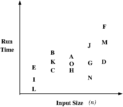
    • Motivated by the need to organize set of instruction-counts over the space of all inputs.
    • Assumes a "reasonable" encoding of inputs, e.g., numbers stored in binary (pages 1055-1057; see also Chapter 2, Garey and Johnson (1979)).
    • Isolate one or more parameters that describe amount of memory used to store input, e.g., length of a given list, the number of vertices in a given graph.
    • Hard to define formally; acquired informally via experience doing time complexity analyses.
    • We will assume where possible that we are dealing with small numbers in the input that fit inside a single computer-memory "word"; hence, the size of numbers in the input need not be a parameter in the input size.
  • Time Complexity
    • Time complexity = instruction-count stated as function of input size.
    • Two general methods to deriving a time complexity function for an algorithm:
      • Compute counts for individual instructions and add together to derive function.
      • "Grow" function by starting at innermost level of nesting in algorithm and working outwards.

      Which method you use depends on the intricacy of the given algorithm.

    • Individual assignment statements count as a single instruction, regardless of the complexity of the expression on the right-hand size.
    • Each type of control-structure has its own rule for counting instructions.
    • while-loop rule: #iter(body + 1) + 1
      • The first "1" in the expression is for the evaluation of the loop-execution condition (to TRUE) for the executions of the loop body, and the second "1" is for the final evaluation of the loop-execution condition (to FALSE) when the loop terminates.
    • Example: while-loop.
    • Example: Example Algorithms #1 and #2 (tc_examples_1.txt)
    • for-loop rule: #iter(body + 2) + 2
      • The first "2" in the expression is for the evaluation of the loop-execution condition (to TRUE) and increment of the index variable for the executions of the loop body, and the second "2" is for the initialization of the index variable before the loop starts and the final evaluation of the loop-execution condition (to FALSE) when the loop terminates.
      • This is very clearly seen if you rewrite a for-loop as the equivalent while-loop.
    • Example: for-loop.
    • Example: Doubly-nested for-loop: the selection sort algorithm (tc_sorting.txt)
  • Worst-Case Time Complexity

    

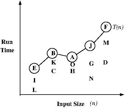
    • Programs involving loops and simple statements naturally give time complexity functions such that every input of a particular size runs in the same time; unfortunately, once we allow arbitrary while and if-then-else statements, different inputs of the same size may run in different times, e,g., sorting algorithms on sorted and unsorted lists of the same length.
    • Need to summarize set of running times for each input size s by a single number. There are three options:
      1. Best-case, e.g., lowest running time over all inputs of size s; easy to compute but not that useful in practice.
      2. Average-case, e.g., average running time relative to some probability distribution over all inputs of size s; useful in practice but hard to compute.
      3. Worst-case, e.g., highest running time over all inputs of size s; easy to compute and useful in practice -- moreover, simplifies analyses (see rule for if-then-else below).
    • Worst-case time complexity functions are both useful and usable; hence, are most commonly in practice.
    • if-then-else-statement rule: max(if-body, else-body) + 1
    • Example: Two analyses of Example Algorithm #3 (tc_examples_1.txt)
    • Example: the linear and binary search algorithms (tc_searching.txt)
    • Example: the bubble and insertion sort algorithms (tc_sorting.txt)
  • Asymptotic notation

    

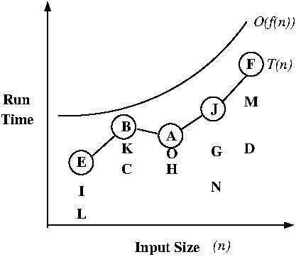
    • Used to smooth and simplify time complexity functions; assumes input size goes out to infinity, and that simplification can be stated in terms of "essential" behavior of function in the limit.
    • What makes a function g(n) a useful and smooth upper bound of a time complexity function f(n) ?
      • g(n) upper-bounds f(n):
        f(n) <= g(n) for all n > 0.

      • g(n) upper-bounds f(n) after initial "bumpy" portion:
        f(n) <= g(n) for all n > n0 for some n0 >= 0.

      • g(n) upper-bounds f(n) after initial "bumpy" portion under arbitrary machine model:
        f(n) <= c * g(n) for all n > n0 for some c > 0 and n0 >= 0.

        This allows (to a degree) for instructions whose running-times differ by a constant multiplicative factor on different machines.

      Note that we have re-derived the definition of big-Oh asymptotic upper-bound notation by combining the mathematical requirements of a useful smoothing function.
    • Asymptotic upper bounds: Big-Oh notation (O(g(n))).
      • Example: T(n) = 3n^2 + 4n + 5 is O(n^2) (big_Oh.txt)
      • One could derive the required constant c by fancy algebra; I prefer to set c to the sum of the positive coefficients -- it's very dirty but it's also quick.
      • Example: T(n) = 3n^2 + 4n + 5 is not O(n) (big_Oh.txt)
      • Try to avoid ludicrously loose upper bounds.
      • Example: T(n) = 2n is O(n^57)
      • Relationship between informal "T(n) is O(g(n))" definition and "O(g(n)) as the set of all g(n)-upper-bounded functions" definition given in textbook; keep the latter in mind, but the former is colloquial CS usage. May stem from algorithm-centric and math-centric views of asymptotic notation, respectively.
    • Asymptotic lower bounds: Omega notation (OMEGA(g(n))).
      • Example: T(n) = 3n^2 + 4n + 5 is OMEGA(n^2) (big_OMEGA.txt)
      • Example: T(n) = 3n^2 + 4n + 5 is not OMEGA(n^3) (big_OMEGA.txt)
      • Try to avoid ludicrously loose lower bounds.
      • Example: T(n) = 2n^57 is OMEGA(n)
    • Asymptotic exact bounds: Theta notation (THETA(g(n))).
      • f(n) is THETA(g(n)) is f(n) is both O(g(n)) and OMEGA(g(n)).
      • Example: Selection sort is both O(n^2) and OMEGA(n^2) and hence THETA(n^2).
    • Three caveats on using asymptotic notation:
      1. How you interpret asymptotic notation depends on how the function T(n) was derived. If T(n) is an exact value for all inputs of a size n, then can say T(n) = O(g(n)) (OMEGA(g(n))) [THETA(g(n))] means "the running time is upper (lower) [exactly] bounded by g(n)"; however, if T(n) is merely an upper bound on the running time (as has been the case in our most recent examples), must be more careful in interpreting OMEGA and THETA statements.
      2. Though it is in a sense an abuse of notation, you will frequently see O(1) or THETA(1) used to indicate an unspecified constant in various expressions.
      3. The rules about combining separate asymptotic-notation expressions are tricky; be VERY careful if you ever do this in your math -- it might be better off to write out the full constant-bounds and work with those, so you don't make mistakes.
    • Guidelines for deriving asymptotic worst-case time complexity functions (non-recursive algorithms)
      • If you have a worst-case time complexity function on hand, the leading term (minus coefficient) is usually the asymptotic worst-case time complexity function.
      • Example: Though the selection, bubble, and insertion sort algorithms run in T(n) = 4n^2 - 2, T(n) = 7n^2 - 3n + 2, and T(n) = 3n^2 - 1 time, respectively, all of these algorithms run in O(n^2) time.
      • As constants associated with different loops and different numbers of embedded simple statements vanish into the leading constant c in the definition of asymptotic notation, can often derive a near-optimal asymptotic worst-case time complexity function by simply multiplying out the number of iterations for each loop in the deepest chain of nested loops.
      • Example: As both the insertion and selection sort algorithms consist of a pair of nested loops, each of which has at most n iterations, both algorithms run in O(n * n) = O(n^2) time.
      • The usual way to handle nested if-then-else statements is to assume the largest sub-case always executes. However, if you have a function describing how often the conditional is true, you may be able to do better, e,g., derivation of O(|V| + |E|) time complexity for breadth-first graph traversal algorithm (see also the second analysis of Example Algorithm #3).

Thursday, September 17 (Lecture #3)
[Section 3.1; Class Notes]

• Background: Time Complexity (Cont'd)
  • Parameterized time-complexity expressions
    • If you are ever confronted with an algorithm which uses operations of unspecified time complexity, build a parameterized time-complexity expression and solve this expression as necessary when you are given the time complexities of those operations.
    • Example: Parameterized versions of Example Algorithms #1 and #2 (tc_param.txt)
    • A particularly useful variant of such expressions are asymptotic worst-case parameterized time-complexity expressions, i.e., simplified big-Oh worst-case versions of parameterized time-complexity expressions.
      • Very useful if algorithm incorporates conditional and/or conditional-loop statements.
      • Derive using the same techniques as you use to derive asymptotic worst-case time complexity expressions modulo the inclusion of variable-terms for unknown operation time complexities.
      • If the term X indicating the execution of the deepest nested loop statements is the same as the term in front of one of unknown-procedure runtimes then ignore X, e.g., O(n^2T(P1) + nT(P2) + n^2) => O(n^2T(P1) + nT(P2)).
      • If the term X indicating the execution of the deepest nested loop statements is greater than the term in front of one of unknown-procedure runtimes then leave X in the expression, e.g., O(n^2T(P1) + nT(P2) + n^3) => O(n^2T(P1) + nT(P2) + n^3).
    • Example: The asymptotic worst-case parameterized time-complexity expressions for Example Algorithms #1 and #2 in the previous example are O(nT(P1)) and O(n^2T(P2) + nT(P1)), respectively.
    • Very nice when you are evaluating an algorithm that uses a set of operations and that set of operations is supported (albeit with different time complexities) by each of a set of data structures -- one derives the parameterized "generic" time complexity for the algorithm and then you derive the time complexity relative to each of the data structures (by filling in the time complexities for the operations relative to that data structure).
    • Also very nice for relating two problems. Suppose a problem P1 can be solved by an efficient, i.e, (asymptotic worst-case) polynomial time, algorithm that invokes a procedure that solves instances of a problem P2, i.e.,

      		    P1(n):
      		      blah blah blah
      		      x = P2(n)
      		      blah blah blah
      		      output z
      		    

      This has several implications:
      • If P2 is efficiently solvable than so is P1 (simply substitute the efficient algorithm for P2 into the algorithm for P1 described above) .
      • If P1 is not efficiently solvable than neither is P2 (if P2 was efficiently solvable, you could substitute that algorithm into the algorithm above for P1 to create an efficient algorithm for P1, which is a contradiction).

      The former is the reason why we create efficient libraries of commonly-called algorithms; as we shall see in the final section of this course, the latter is the basis for showing that a problem does not have an efficient algorithm.

• Potential exam questions
• Algorithm Design Techniques
  • Combinatorial optimization problems redux
    • Each solution associated with an instance of a combinatorial optimization problem has a cost, and we want the solutions of optimal (min/max) cost over the whole solution space.
      • Any time you have a problem of the form "Find the best X" where X is some discrete structure, chances are you're dealing with a combinatorial optimization problem.
    • Distinguish several types of solutions:
      • Candidate solutions = all possible solutions to the instance, e,g., all possible edge-sequences of a given graph that start with vertex u and end with vertex v.
      • Viable solutions = all potentially optimal candidate solutions, e.g., all edge-sequences of a given graph that are paths between vertices u and v.
      • Optimal solutions = those viable solutions that have optimal value relative to the cost function over the set of viable solutions, e.g., all paths in a given graph between vertices u and v that have the smallest number of edges over the space of all such paths.
    • Each such problem instance has a combinatorial, i.e., exponential in instance size, candidate (and often viable) solution space -- the job of an algorithm is to to find the optimal solutions in this space (of which there will always be at least one).
    • Sometimes, you can't generate viable solutions -- you have to generate all candidate solutions and check viability along the way.
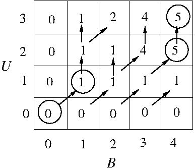
    • Example: The 0/1 Knapsack problem
      • Candidate solutions = subsets of U.
      • Viable solutions = subsets of U whose summed size is <= B.
      • Optimal solutions = subsets of U whose summed size is <=B and whose summed value is maximum over the space of viable solutions.
      • Each subset U' can be modeled as a binary vector of length |U| (v_i = 1 (0) => item i is (not) in U'); hence, there are 2^{|U|} candidate solutions for any instance of 0/1 Knapsack.
    • Sometimes, you can generate viable solutions up front -- this depends in part on your ingenuity.
    • Example: The Longest Common Subsequence problem

      Longest common subsequence (LCS)
      Input: Two strings s, s' over an alphabet Sigma.
      Output: All strings s'' over Sigma such that s'' is a subsequence of both s and s' and the length of s'' is of is maximized over the solution space.

      • Candidate solutions = all possible strings over alphabet Sigma of length <= min(|s|,|s'|).
      • Viable solutions = all subsequences of the shorter given string.
      • Optimal solutions = all subsequences of the shorter given string that are also subsequences of the longer given string and have the maximum length over the space of viable solutions.
      • Each subsequence s'' can be modeled as a binary vector of length min(|s|,|s'|) (v_i = 1 (0) => symbol i is (not) included in the subsequence); hence, there are O(2^{min(|s|,|s'|)}) viable solutions for any instance of LCS (note that this worst case only occurs if each symbol in s and s' only occurs once).
    • Sometimes even the set of viable solutions is dauntingly large (like, REALLY large).
    • Example: The Minimum Spanning Tree problem
      Minimum spanning tree (MST)
      Input: An edge-weighted graph G = (V, E, w).
      Output: All spanning trees T of G, i.e., trees that connect all vertices in G, such that the sum of the weights of the edges in T is minimized over the solution space.
      • Candidate solutions = all (|V| - 1)-sized subsets of the edges of G.
      • Viable solutions = all (|V| - 1)-sized subsets of the edges of G that are spanning trees of G.
      • Optimal solutions = all spanning trees of G that have minimum summed edge-weight over the space of viable solutions.
      • By Cayley's Theorem, a graph G = (V, E) has O(|V|^{|V| - 2}) spanning trees (the worst case here is when G is a complete graph); hence, there are O(|V|^{|V| - 2}) viable solutions for any instance of MST.
    • Can solve combinatorial optimization problems by looking at all (candidate/viable) solution and saving those of the optimal cost (which we can determine on the fly by saving those solutions with the best cost we've seen so far at any point in the enumeration of all solutions).
    • This is inherently inefficient given the exponential sizes of the (candidate/viable) solution spaces involved. Can we do better?
      • We most certainly can. Consider MST; though the set of viable solutions for each instance of MST is potentially exponentially large, we can solve all instances of MST in low-order polynomial time.
      • How good we can do algorithm-wise depends on how much of the (candidate/viable) solution space our algorithm can ignore. Over the next 8 lectures, we'll examine a set of techniques for doing this whose applicability depend on some fairly simple properties of problem solution-spaces.
  • Combinatorial Solution-Space Trees (Sections 9.1-9.7, B&B)
    • The most basic approach to solving combinatorial optimization problems in which we are interested in finding a subset SS' of a given set SS such that c(SS') is optimal relative to some solution-evaluation function c().
    • As a first step, simplify generation of solutions for a problem instance by using a combinatorial solution-space tree (CST).
      • In such a tree, internal nodes are partial solutions and the full solutions labeling the leaves comprise the solution space.
      • The simplest such trees are binary, and each of the |SS| levels in the tree effectively decides whether or not to add a particular item in SS to the solution
    • Example: A CST for an instance of 0/1 Knapsack in which SS = U = {X, Y, Z} and |SS| = |U| = 3:

      

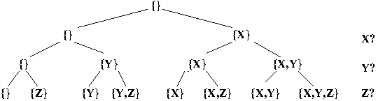
  • One can vary the items added at each CST level to construct different types of solutions for different problems.
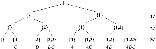
  • Example: A CST for an instance (s = ABAACA, s' = ADC) of Longest common subsequence in which SS = {1, 2, 3}, i.e., positions in the shorter given string (in this case, s') and |SS| = |s'| = 3:

    

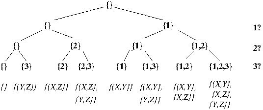
  • Example: A CST for an instance (I = {X, Y, Z}, S = {{X, Y}, {X, Z}, {Y, Z}}) of Set cover (see Programming Problem #1) in which SS = {1, 2, 3}, i.e., the numbers of the subsets of I in S, and |SS| = |S| = 3:

    

Tuesday, September 22 (Lecture #4)
[Class Notes]

• Algorithm Design Techniques (Cont'd)
  • Combinatorial Solution-Space Trees (Cont'd)
    • Can traverse such a tree and examine all of its leaves using depth-first search (DFS) or breadth-first search (BFS). Only those leaves corresponding to viable solutions are important.
    • Example: Viability conditions for 0/1 Knapsack, LCS, and MST.
      • Do items in partial solution fit in knapsack? (0/1 Knapsack)
      • Is partial solution string a subsequence of both given sequences? (LCS)
      • Do edges in partial solution form a forest? (MST)
    • As a second step, decrease space requirements by operating on an implicit CST, i.e., generate tree nodes as necessary during traversal.
    • ALGORITHM: DFS-based traversal of implicit CST (minimization version) [PROGRAMMING PROBLEM #1]

       1. DFS-I(i, sol)
       2.    if (i == n + 1)
       3.       if (viable (sol))
       4.           return(cost(sol))
       5.       else
       6.           return(INFINITY)
       7.   else
       8.       return(min(DFS-I(i + 1, sol),
       9.                  DFS-I(i + 1, sol U item[i])))
      

      • Initial call: DFS-I(1, empty set)
      • Note that n is the number of items in the set in the instance; hence "i == n + 1" means that you have reached a leaf in the CST.
    • ALGORITHM: BFS-based traversal of implicit CST (minimization version).

       1. BFS-I()
       2.    Q = {(1, empty set)}
       3.    best = INFINITY
       4.    while not empty(Q)
       5.      (i, sol) = pop(Q)
       6.      if (i == n + 1)
       7.         if (viable(sol))
       8.            best = min(best, cost(sol))
       9.      else
      10.         push(Q,(i + 1, sol))
      11.         push(Q,(i + 1, sol U item[i]))
      12.    return(best)
      

    • Modifications:
      • To make the above work for maximization problems, change min to max and INFINITY to -INFINITY.
      • To obtain optimal solutions, the simplest way is to run a second tree-traversal that takes the optimal cost produced previously as a parameter and stores / prints all viable solutions with that cost.
    • Example: Execution of DFS-based traversal of implicit CST for 0/1-Knapsack when U = {X,Y,Z}, s(X) = 4, s(Y) = 2, s(Z) = 1, v(X) = 4, v(Y) = 5, v(Z) = 3, and B = 4:

      

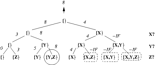
      Note that optimal leaf-solutions are circled and non-viable leaf-solutions are enclosed in dashed boxes.

    • This is all well and good; however, we are still looking at every node in the tree, and as this tree is of exponential size, our algorithm runs in exponential time. Can we do better? Yes we can!
    • As a third step, where possible, use information about partial solution viability and potential optimality to terminate search of unfeasible subtrees of the CST (dynamic pruning).
      • Traditionally, DFS + dynamic pruning is known as backtracking and BFS + dynamic pruning is known as branch and bound.
      • Dynamic pruning works in CST because all "full" candidate solutions that incorporate a particular particular partial solution are leaves in the subtree rooted at the node corresponding to that partial solution; hence, non-viability / non-potential-optimality of a partial solution implies the non-viability / non-potential-optimality of all solutions in the subtree rooted at the node corresponding to that partial solution!
    • Example: Potential optimality conditions for 0/1 Knapsack, LCS, and MST.
      • Does sum of values of items in partial solution plus sum of values of all remaining items that could be added exceed the value of the best solution seen so far? (0/1 Knapsack)
      • Does the length of the partial solution string plus the length of the string of all remaining characters that could be added exceed the length of the best solution string seen so far? (LCS)
      • Is the sum of the weights of the edges in the partial solution less than the cost of the best solution found so far? (MST)
    • ALGORITHM: DFS-based traversal of implicit CST + dynamic pruning (minimization version).

       1. DFS-IP(i, sol, best)
       2.    if (not viable(sol)) or (best < cost(sol))
       3.       return(INFINITY)
       4.    else if (i == n + 1)
       5.       best = min(best, cost(sol))
       6.       return(cost(sol))
       7.    else
       8.       return(min(DFS-IP(i + 1, sol, best),
       9.                  DFS-IP(i + 1, sol U item[i], best)))
      

      • Initial call: DFS-IP(1, empty set, BEST) where BEST is an object encoding the integer INFINITY.
      • Note that variable BEST is passed by reference, e.g., it is a pointer to an integer; if it is passed by value, the value of BEST is not saved from any of the leaf-evaluations.
    • ALGORITHM: BFS-based traversal of implicit CST + dynamic pruning (minimization version).

       1. BFS-IP()
       2.    Q = {(1, empty set)}
       3.    best = INFINITY
       4.    while not empty(Q)
       5.       (i, sol) = pop(Q)
       6.       if (viable(sol) and (cost(sol) < best))
       7.	     if (i == n + 1)
       8.             best = min(best, cost(sol))
       9.          else
      10.             push(Q,(i + 1, sol))
      11.             push(Q,(i + 1, sol U item[i]))
      12.    return(best)
      

    • Example: Execution of DFS-based traversal of implicit CST for 0/1-Knapsack with dynamic pruning based on non-viability when U = {X,Y,Z}, s(X) = 1, s(Y) = 3, s(Z) = 2, v(X) = 1, v(Y) = 4, v(Z) = 2, and B = 3:

      

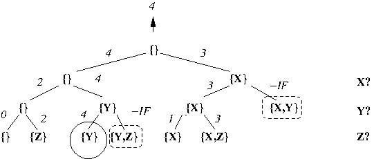
      Note that optimal solutions are circled and non-viable solutions are enclosed in dashed boxes.

    • Example: Execution of DFS-based traversal of implicit CST for 0/1-Knapsack with dynamic pruning based on both non-viability and non-potential optimality when U = {X,Y,Z}, s(X) = 1, s(Y) = 3, s(Z) = 2, v(X) = 1, v(Y) = 4, v(Z) = 2, and B = 3:

      

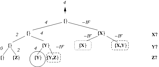
      Note that optimal solutions are circled and non-viable (non-potential optimal) solutions are enclosed in dashed (dotted) boxes.

    • Such tricks can (but may not always) drastically reduce actual running times for CST traversal.
    • Applicatiions: Inference in Propositional logic (PL)
      • Sentences in PL can be atomic sentences consisting of a single Boolean literal, i.e., True, False, or propositional symbol, e.g., P, Q, R, or complex sentences built up using logical connectives, e.g., not, and, or, => (implies), <=> (if and only if), and parentheses.
      • Given a knowledge base KB and a sentence s in PL over propositional symbol set S, we want to determine if KB entails s, i.e., for all possible truth-assignments to the symbols in S (that is, all possible models for S) check that s is true for every truth-assignment for which KB is true.
      • EXAMPLE: The basic complete model-tree for the sentence ``not A or B" in propositional logic relative to variable-ordering B -> A and value-ordering F -> T.

        

        Note that all nodes in the tree corresponding to models that make the given sentence true have been circled.

      • Can do model checking via backtracking with (massive number of) dynamic pruning heuristics on the complete model-tree (the Davis-Putnam-Logeman-Loveland (DPLL) algorithm).
      • A variety of scale-up enhancements to the DPLL algorithm allow modern inference engines to tackle input instances with tens of millions of variables.
    • Food for Thought:
      1. Can we do better in practice runtime-wise if we only require one optimal solution? How about in the worst case?
      2. Can we do better in practice runtime-wise if we require all optimal solutions? How about in the worst case?
  • Potential exam questions
  • The CST approach to solving combinatorial optimization problems assumes nothing about the structure of the solution space for an instance. If we did have such knowledge, can we do better?
  • There are other types of computation trees besides CST. There are, for example, the trees associated with recursive computations, in which nodes represent individual recursive algorithm calls on subproblems of smaller size. Such a recursive-call tree is also called a recursive decomposition.
  • Characteristics of recursive decomposition:
    • Can decompose instance of problem into smaller instance of the same problem, i.e., subproblems.
    • At any point in the computation, may be several choices for decomposition.
  • Problems that are solvable by recursive decomposition have the optimal substructure property, i.e, an optimal solution for an instance of the problem can be constructed using optimal solutions for instances of that problem that are of smaller size (subproblems)..
  • Our remaining algorithm design techniques will be applicable if a problem's recursive decomposition satisfies additional properties.
  • Divide-and-Conquer (D&C)
    • Applies if a problem has recursive decomposition in which each subproblem occurs only once, i.e., the subproblems do not repeat.
    • Will typically only be efficient if the depth of recursion is logarithmically bounded, thus ensuring that the total number of recursive calls is polynomially bounded.
    • Example: Binary search in a sorted list
      • Look at midpoint in current list; if wanted element is not there, repeat midpoint search on lower (upper) half sublist if wanted element is less (greater) than the midpoint.
      • Each sublist is searched only once; moreover, can only halve a list of n elements log_2 n times.
      • Can be done in O(log_2 n) time.
    • Example: Merge sort (Section 2.3.1)
      • Recursively halve a list until sublists have single elements, and on return, merge sorted sublists in linear time.
      • Each sublist is sorted only once; moreover, can only halve a list of n elements log_2 n times.
      • Can be done in O(n log_2 n) time.
    • Example: Strassen's matrix multiplication algorithm (Section 4.2)
      • Can rephrase multiplication of two n x n matrices by recursively decomposing each matrix into four n/2 x n/2 submatrices and intricately multiplying and adding these submatrices.
      • Each submatrix is multiplied only once; moreover, can only halve an n x n matrix log_2 n times.
      • This still requires O(n^3) but if we apply a more intricate still submatrix multiplication / addition scheme due to Strassen, we get a runtime of O(n^{log_2 7}).

Tuesday, September 22

• In-class Exam #1 Notes
  I've finished making up the first in-class exam. The exam will be closed-book and written in-class on paper (please bring your own pens). It will be 75 minutes long and has a total of 50 marks (this is not coincidental; I have tried to make the number of marks for a question approximately equal to the number of minutes it should take you to do it in the best case). The exam will cover material in all course lectures up to and including Lecture #6 (Topics 2-4 in the potential exam question list). There will be four questions:
  1. Time complexity I [Topic 2] (3 parts / 9 marks)
  2. Time complexity II [Topic 2] (3 parts / 9 marks)
  3. Algorithm Design Techniques I [Topic 3] (2 parts / 20 marks)
  4. Algorithm Design Techniques II [Topic 4] (1 part / 12 marks)

  I hope the above helps, and I wish you all the best of luck with this exam.

Thursday, September 24 (Lecture #5)
[Sections 2.3.1, 4.2, and 15.3-4; Class Notes]

• Algorithm Design Techniques (Cont'd)
  • The relationship between CST and Divide-and-Conquer algorithms:

    				Optimal
    			      Substructure?
    		             /          \
    			    / YES        \ NO
    	                   /              \
    	                 D&C              CST
    	      

  • How can we exploit the optimal substructure problem if subproblems are repeated?
  • Dynamic Programming
    • Applies if a problem has a recursive decomposition and the number of distinct problems is bounded and can be organized in some n-dimensional table.
    • Example: Computing Fibonacci numbers
      • Recurrence (recursive + base cases)
        • Fib(i) = ith Fibonacci number, i >= 1
        • Fib(i) = Fib(i - 1) + Fib(i -2) for i > 2.
        • Fib(1) = Fib(2) = 1
      • ALGORITHM: Fibonacci numbers (Recursive)

         1. FibR(n)
         2.    if ((n == 1) || (n == 2))
         3.       return(1)
         4.    else
         5.       return(FibR(n - 1) + FibR(n - 2))
        

      • Recursive-calls tree: 2^{n/2} - 1 <= Tree Size <= 2^{n} - 1
      • The problem here is that subproblems are being repeated; perhaps the recursive algorithm can keep track of what subproblems have been solved by storing those values in a table and look these up as necessary? An algorithm that does this is called a memoized algorithm.
      • ALGORITHM: Fibonacci Numbers (Memoized (Recursive))

         1. InitFibT(n,FibT)
         2.    Allocate n-element table and assign to FibT
         3.    FibT[1] = FibT[2] = 1
         4.    for (i = 3; i <= n; i++)
         5.       FibT[i] = INFINITY
        
         6. FibM(n, FibT)
         7.    if (FibT[n] == INFINITY)
         8.       FibT[n] = FibM(n - 1, FibT) + 
         9.                 FibM(n - 2, FibT)
        10. return(FibT[n])
        

      • This table idea was pretty neat. In fact, do we really need the recursion anymore? Let's just fill out the table!
      • ALGORITHM: Fibonacci Numbers (Dynamic programming (Iterative))

         1. FibI(n)
         2.    if ((n == 1) || (n== 2))
         3.       return(1)
         4.    else
         5.       Allocate n-element table FibT
         6.       FibT[1] = FibT[2] = 1
         7.       for (i = 3; i <= n; i++)
         8.           FibT[i] = FibT[i - 1] + FibT[i - 2]
         9.       return(FibT[n])
        

    • If we are lucky, there are a polynomial number of distinct subproblems. If we are really lucky, we can use the recurrence to solve these subproblems in a "bottom up" rather than a "top down fashion", solving the smallest subproblems first and solving progressively larger subproblems until we solve the original problem instance.
    • Dynamic programming (DP) => table-driven, bottom-up recursive decomposition algorithms!
    • The Dynamic Programming Cookbook:
      • Step 1: Find a recurrence / recursive decomposition for the problem of interest; this includes approprtiately defining the problem of interest.
        • The subproblems typically ask for the cost of an optimal solution to a subproblem.
      • Step 2: Lay out the distinct subproblems in a table.
      • Step 3: Fill in the base-case values in the table.
      • Step 4: Run the recurrence "in reverse" / in a bottom-up fashion, using smaller solved subproblems to solve larger subproblems, until the table is filled in.
        • This fillin typically includes information about the choice(s) made in solving a subproblem (backpointers) that is used in Step 5.
      • Step 5: Use traceback on backpointers starting from the optimal-cost table entry for the original subproblem of interest to reconstruct one or more optimal solutions for that problem.
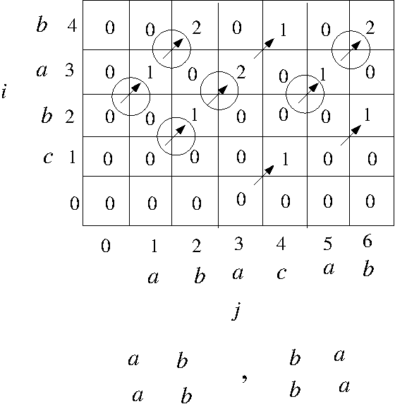
    • Example: DP algorithm for Longest Common Subsequence (LCS)
      • Recursive decomposition
        • Given strings s and s' over some alphabet, D(i,j) = length of longest common subsequence of first i characters of s and first j characters of s'.
        • Two recursive cases:
          1. ith character of s and jth character of s' are the same.
          2. jth character of s and jth character of s' are different.
      • Recurrence (recursive + base cases)
        • Case 1: D(i,j) = D(i - 1, j - 1) + 1 for i, j > 0
        • Case 2: D(i,j) = max(D(i, j - 1), D(i - 1, j)) for i, j > 0
        • D(i,0) = D(0,j) = 0 for i, j >= 0
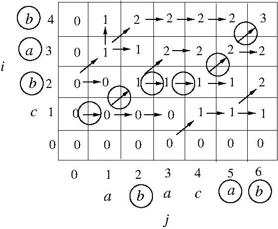
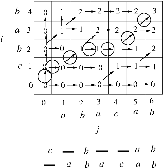
      • Matrix fill-in (including backpointers) for deriving length of longest common subsequence.
        • Rectangular (m + 1) x (n + 1) matrix; fill-in proceeds from cell (1,1) row-wise, column-wise, or anti-diagonal-wise.
        • Fill-in of an individual cell involves consulting filled-in cells in the 3-cell "overhang" to left and above of that cell.
        • Backpointer cells have value 1, 2, or 3 depending on which recursive (sub)case was invoked.
      • Derivation of an LCS involves matrix-fill in get the length of a longest common subsequence followed by traceback from cell D(|s|,|s'|) for deriving a longest common subsequence.

Tuesday, September 29 (Lecture #6)
[Section 15.4]

• Algorithm Design Techniques (Cont'd)
  • Dynamic Programming (Cont'd)
    • Example: DP algorithm for Longest Common Subsequence (LCS) (Cont'd)
      • Example: LCS of s = cbab and s' = abacab

        

        Observe that the reconstructed LCS is bab (matching characters in s and s' as well as the traceback path to derive this subsequence are indicated by circled elements).

      • Example: LCS of s = ABCBDAB and s' = BDCABA (page 395).
      • DP algorithm (table fill-in (page 394) + traceback (page 395))
      • Time complexity of matrix fill-in: (# cells) x (#choices per cell) x (max # subproblems per choice) = (m + 1)(n + 1) x 2 x 2 = O(mn)
      • Time complexity of traceback = O(m + n) [longest possible backpointer path from D[|s|,|s'|] to D[0,0]].
      • Space complexity: # cells = (((m + 1) x (n + 1)) = O(mn)
      • Food for thought:
        1. How does the above change if we want to enumerate all possible LCS of s and s'?
        2. Can we do better spacewise if all we want is the length of an LCS of s and s'?
        3. Can we do better spacewise when obtaining a single LCS of s and s'?
        4. How does the above change if there are different degrees of symbol identity, e.g., identical a's are worth more than identical b's or c's?
        5. How does the above change if we want to compute longest common substrings?
      • Applications: Pairwise Alignment of Biological Molecular Sequences
        • We ignored backpointers to non-matching symbols in our DP LCS algorithm above. However, if we are dealing with a pair of similar molecular sequences (DNA or protein) in two species, a visualization of all matching and non-matching symbols in the backpointer path (a < b>pairwise alignment) can help in understanding how the sequences have evolved since the divergence of the two species involved from their last common ancestor
          • Non-matching charcters in an alignment are indicated by dashes (gaps). As it is not obvious in a pairwise alighment if a gap is a result of symbol insertion or deletion during sequence evolution, gaps are also known as indels.
        • Example: A possible pairwise alignment of DNA sequences s = TAACG and s' = ATACAG.

          

        • Let M(x,y) be the similarity of characters x and y. Consider the following three options for pairtwise alignment of a given string s relative to a given string ` s':
          1. Pairwise LCS alignment (Section 11.6.2, Gusfield (1997))
             • Focus on matching characters.
             • Interpret D(i,j) as length of longest common subsequence of prefix i of s and prefix j of s'.
             • Recurrence is D(i,j) = Max{D(i, j - 1), D(i - 1,j), D(i - 1, j - 1) + M(s(i),s'(j))}, where M(i,j) = 1 if s(i) = s'(j) and 0 otherwise, with boundary conditions D(i,0) = D(0,j) = 0.
             • Traceback starts at D(m,n) and goes back to D(0,0); note that each traceback-path from D(m,n) to D(0,0) corresponds to a longest common subsequence.
             • Example: A pairwise LCS alignment of sequence s = cbab and s' = abacab when M(x,y) = 1 if x = y and 0 otherwise.

               

          2. Global pairwise alignment (Section 11.3, Gusfield (1997))
             • Look for best alignment of all of s with all of s'.
             • Interpret D(i,j) as best alignment between prefix i of s and prefix j of s'.
             • Recurrence is D(i,j) = OPT{D(i, j-1) + C(indel), D(i - 1,j) + C(indel), D(i - 1, j - 1) + M(s(i),s'(j)) with boundary conditions D(i,0) = i * C(indel) and D(0,j) = j * C(indel), where C(indel) is the cost of an indel relative to any symbol in an alignment.
             • Traceback starts at D(m,n) and goes back to D(0,0).
             • Example: A global pairwise alignment of sequence s = cbab and s' = abacab when M(x,y) = 1 if x = y and -1 otherwise and C(indel) = -2.
          3. Local pairwise alignment (Section 11.7, Gusfield (1997))
             • Look for the best alignment of a region of s with a region of s'.
             • Interpret D(i,j) as best alignment over all suffixes of prefix i of s and all suffixes of prefix j of s'.
             • Recurrent portion same as for global alignment with inclusion of leading 0-term; boundary conditions same as pairwise LCS alignment(D(i,0) = D(0,j) = 0).
             • Traceback starts at any maximum-value cell in the table and continues back until a 0-value cell is reached.
             • Change in recurrence allows start of optimal alignment at any points in both strings and traceback procedure allows termination of region at any points in both strings.
             • Example: A local pairwise alignment of sequence s = cbab and s' = abacab when M(x,y) = 1 if x = y and -1 otherwise and C(indel) = -2.

               

             There many other types of alignment, e.g., pairwise semi-global, multi-sequence.

    • Another important characteristic of problems whose optimal substructure can be exploited by dynamic programming (and indeed by divide-and-conquer and greedy algorithms as well) is subproblem independence, i.e., solutions to subproblems do not share resources. This is important because subproblem solutions can only be combined if they are independent.
    • Example: The existence (impossibility) of dynamic programming algorithms for the unweighted shortest (longest) simple path problems in directed graphs (pp. 381-384).
      • Recall that in a simple path, vertices cannot repeat.
      • USSP has the optimal substructure property.
        • Consider a shortest path p between any two vertices u and v incorporating an intermediate vertex w (which may be u or v); this can be decomposed into subpaths p1 and p2 between u/w and w/v, respectively.
        • If p is a shortest path between u to v then then p1 must be a shortest path between u and w (proof by contradiction: if there was a shorter path p` between u and w, it could be combined with p2 to create a path shorter than p, which contradicts the optimality of p).
        • An analogous argumnent establishes the optimality of p2.
        • This recursive decomposition is the basis of a shortest-path algorithm we will examine later in this course.
      • ULSP does not have the optimal substructure property.
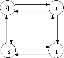
        • Consider the following graph G:

          

          Observe that the longest simple path between q and t is q-r-t, but the longest simple path between q and r (q-s-t-r) cannot be combined with the longest simple path from r to t (r-q-s-t) to get the longest simple path from q to t because vertices repeat in these two paths.
        • Unlike USSP, subproblems in ULSP are not independent, as they share resources (in this case vertices) and cannot be patched together to create solutions to larger problems.
      • ULSP does not have the optimal substrtucture property and hence does not have cool DP or Divide-and-Conquer algorithms; however, might there be another route to polynomial-time solvability for ULSP? As we shall see later in this course, the answer to this question is "probably not".
  • Potential exam questions

Thursday, October 1

• In-class Exam #1

Tuesday, October 6 (Lecture #7)
[Section 15.2; Class Notes]

• Went over In-class Exam #1.
• Algorithm Design Techniques (Cont'd)
  • Dynamic Programming (Cont'd)
    • Note that the dynamic programming algorithms we have seen so far are only useful because they have a polynomially-bounded number of subproblems -- this need not always be the case.
    • Example: DP algorithm for 0/1 Knapsack
      • Recursive decomposition
        • V(i,j) = summed of value of optimal knapsack load with size <= j, 0 <= j <= B, composed of selection from first i, 0 <= i <= |U|, items of U.
        • V(i,j) depends on whether or not item i can be added to a knapsack of size j.
      • Recurrence (recursive + base cases)
        • V(i,j) = max{V(i - 1,j), V(i - 1, j - s(u_i)) + v(u_i)}
          • First term: Cannot add item i to knapsack.
          • Second term: Can add item i to knapsack.
        • V(i,0) = V(0,j) = 0 (intuitively, both the knapsack of capacity 0 and the knapsack with 0 items to include in it have value 0); all other V(i,j) consulted by the recurrence are out of bounds of the table are assumed to have value -INFINITY.
      • Matrix fill-in (including backpointers) for deriving value of optimal knapsack.
        • Rectangular (|U| + 1) x (B + 1) matrix; fill-in proceeds from cell (1,1) row-wise, column-wise, or anti-diagonal-wise.
        • Fill-in of an individual cell involves consulting cell immediately above (V(i - 1,j)) and cell back one row to the left (V(i - 1, j - s(u_i))).
        • Backpointer matrix cells have value 1 or 2, depending on which recursive case was invoked.
      • Example: Optimal solution for 0/1 Knapsack when U = {u1,u2,u3}, s(u1) = 1, s(u2) = 3, s(u3) = 2, v(u1) = 1, v(u2) = 4, v(u3) = 2, and B = 4:

        

        Note that diagonal backpointers go back in the row and not necessarily to that backpointer's origin-cell. Observe that the above yields the optimal solution {u1,u2} with value 5.

      • Time complexity of matrix fill-in: (# cells) x (#choices per cell) x (max # subproblems per choice) = ((|U| + 1) x (B + 1)) x 2 x 1) = O(|U|B)
      • Time complexity of traceback = O(|U| + B) [longest possible backpointer path from V[|U|,B|] to V[0,0]].
      • Space complexity: # cells = ((|U| + 1) x (B + 1)) = O(|U|B)
      • Wait a minute ... this isn't a polynomial-time (or space) algorithm, because |U|B is not a polynomial of the input size (|U| + log B). What we actually have here is an exponential time algorithm!
      • Food for thought:
        1. How does the above change if we want to enumerate all possible optimal 0/1 Knapsaack solutions?
        2. Can we do better spacewise if all we want is the value of the optimal solution?
        3. Can we do better spacewise when obtaining a single optimal solution?
        4. Can we do better if we know that the value of B is bounded by some polynomial function in |U|?
      • Additional caveats:
        • DP is not necessarily better than CST!
          • CST for 0/1 Knapsack (DFS + pruning): O(2^{|U|}|U|) time, O(|U|) space.
          • DP for 0/1 Knapsack: O(|U|B) time and space.
          • CST always bettrer wrt space and better wrt time when |U| < log B.
        • There may be no "best" algorithm for a problem -- rather there are only algorithms that are the best relative to particular ranges of input-parameter values. It is therefore crucial for a human algorithm designer to both find those ranges of input-parameter values that characterize a given application AND reason about which algorithms are most appropriate for that application.
          • Sounds oddly like system requirements gathering and system architecture design in software engineering, yes?
          • Such activities are for now beyond automatic coding platforms like chatGPT and may point to roles only humans can play in future in algorithm and software system creation.
  • The relationship between CST, DP, and Divide-and-Conquer algorithms:

    				Optimal
    			      Substructure
    			          AND
                                  Independent
                                  Subproblems?
    		             /          \
    			    / YES        \ NO
    	                   /              \
    	              Repeated            CST
    		    Subproblems?
                       /            \
                      / YES          \ NO 
                     /                \
                   DP                  D&C
    	      

  • Potential exam questions

Thursday, October 8 (Lecture #8)
[Sections 16.1-16.2; Class Notes]

• Algorithm Design Techniques (Cont'd)
  • Dynamic programming and divide-and-conquer algorithms have enabled us to make many apparently difficult problems solvable in low-order polynomial time. Can we do still better? In certain cases, it seems that we can.
    • Consider binary search; it is a particularly interesting example of a D&C algorithm in which there is, at each point in the computation, at most 1 choice and 1 subproblem to be solved. In this case, the recursive computation collapses to a path of recursive calls from the "root" problem to a "leaf" subproblem.
    • The subproblem structure for binary search is unusually simple, in that a choice can be made before the subproblem is solved, i.e., the choice can be made in a top-down, locally optimal (greedy) manner. Compare this with other listed D&C and dynamic programming algorithms, which solve subproblems in a bottom-up manner and make choices only after all necessary subproblems have been solved.
    • As we we shall see, exploiting such greedy choices, while implementable succinctly in code, comes at the cost of increasingly complex proofs of correctness.
  • Greedy Algorithms
    • Example: The Activity Selection problem
      • Suppose we have set S = {a1, a2, ..., an} of activities that use a resourse such as a lecture room, where each activity ai has associated start and finish times si and fi such that 0 <= si < f1 < INFINITY.
        • We will assume that the activities in S are sorted in increasing order by finishing time, i.e., fi <= fj for i < j.
      • Two activities ai and aj are compatible if they do not overlap in time, i.e., fi <= sj.
      • The activity selection problem looks for the largest set of mutually compatible activities.
      • Example: Consider the following set of 11 activities (page 415):

        i  |   1   2   3   4   5   6   7   8   9  10  11
        ------------------------------------------------
        si |   1   3   0   5   3   5   6   8   8   2  12
        fi |   4   5   6   7   9   9  10  11  12  14  16
        

        The activities in the subset {a3, a9, a11} are all mutually compatible, but the largest such subset is {a1, a4, a8, a11}.
      • Recursive decomposition
        • Sij = the set of activities that start when or after ai finishes and finish before or when aj starts (we will assume "dummy" left and right endpoint activities a0 and a(n+1)).
        • c(i,j) = maximum number of mutually compatible activities in Sij.
          • Note that the value we need to solve the activity selection problem is c(0,n+1)!
        • Value c(i, j) for i < j is the sum of the values of the best two-way split of activity subsequence i through j plus 1 (that is, the best split at some solution-included activity k for i <= k < j).
      • Recurrence (recursive + base cases)
        • c(i,j) = max{i <= k < j} c(i,k) + c(k,j) + 1 if Sij is not empty.
        • c(i,j) = 0 if Sij is empty.
        • This looks an awful lot like the recurrence we derived for MCP, doesn't it?
      • Matrix fill-in (including backpointers) for deriving the optimal activity selection.
        • Ragged-bottom pyramid / B2 bomber shape matrix; fill-in proceeds from left to right in ascending rows.
        • Fill-in of an individual cell involves consulting filled-in cells in the "boomerang" hanging off that cell.
        • Backpointer matrix cells have value k at which matrix sequence i .. j split into activity subsequences i .. k and (k + 1) .. j.
      • Can we do better? In particular, do we have to evaluate all subproblem-pairs induced by a choice ak from S(i,j), or can we get away with a single ak-choice and subproblem?
        • It turns out that we can -- to get an optimal solution for S(i,j), greedily pick the activity am from S(i,j) with the earliest finishing time -- we are then left with the subproblem S(m,j)! (Theorem 16.1).
      • This gets even better -- note that instead of solving all S(i,j) in the bottom-up manner described above, we start with S(0,n+1) and solve directly in an iterative (and not recursive) top-down manner!
      • ALGORITHM: Activity Selection (Greedy (Recursive)) (page 419)
      • ALGORITHM: Activity Selection (Greedy (Iterative)) (page 423)

         1. ActSelGI(s, f)
         2.   n = s.length
         3.   A = {a1}
         4.   k = 1
         5.   for m = 2 to n do
         6.      if s(m) >= f(k) then
         7.         A = A u {am}
         8.         k = m
         9.   return A
        

      • Example: Derivation of an optimal activity selection in the example given above by the greedy algorithm (page 420).
      • Time AND space complexity (assuming we do not have to sort the activities in S by finishing time) = O(n).
      • Food for thought:
        1. Can we do better spacewise when obtaining a single optimal solution?
        2. Can we do better spacewise if all we want is the value of the optimal solution?
        3. How does the above change if we want to enumerate all possible optimal activity selections?
    • The Greedy Algorithm Cookbook [long form] (page 423)
      1. Determine the optimal structure of the problem, i.e., derive the recursive decomposition.
      2. Develop a recursive solution, i.e., derive the recurrence.
      3. Show that if we make the greedy choice then only one subproblem remains.
      4. Prove that it is always safe to make the greedy choice, i.e., that the greedy choice will always be part of some optimal solution.
      5. Develop a recursive algorithm that implements the greedy strategy.
      6. Convert the recursive algorithm to an iterative algorithm

References

Unless otherwise stated, all references above are to Cormen et al. (2009).
• Aaronson, S. (2007) "The Limits of Quantum." Scientific American, 298(3), 62-69.
• Ausiello, G., Crescendi, G. Gambosi, V. Kahn, A. Marchetti-Spaccamela, and M. Protasi (1999) Complexity and Approximation of Combinatorial Approximation Problems and their Approximability Properties. Springer; Berlin.
• Brassard, G. and Bratley, P. (1996) Fundamentals of Algorithmics. Prentice-Hall; Englewood Cliffs, NJ. [Abbreviated above as B&B]
• Bernstein, A., Nanongkai, D., and Wulff-Nilsen, C. (2025) "Negative-weight single-source shortest paths in near-linear time." Communications of the ACM, 68(2), 87-94 Cesati, M. and Wareham, H.T. (1995) "Parameterized Complexity Analysis in Robot Motion Planning." In Proceedings of the 25th IEEE International Conference on Systems, Man, and Cybernetics: Volume 1. IEEE Press; Los Alamitos, CA. 880-885.
• Cook, S. (1971) The complexity of theorem proving procedures. In Proceedings of the Third Annual ACM Symposium on Theory of Computing. ACM Press; New York. 151-158.
• Cormen, T.H., Leiserson, C.E., Rivest, R.L., Stein, C. (2009) Introduction to Algorithms. Third Edition. The MIT Press; Cambridge, MA. [Abbreviated above as CLRS]
• Daily, W. (2022) "Point/Counterpoint: On the Model of Computation." Communications of the AC M, 65(9), 30-32. [PDF]
• Downey, R.G. and Fellows, M.R. (1999) Parameterized Complexity. Springer-Verlag; Berlin.
• Garey, M.R. and Johnson, D.S. (1979) Computers and Intractability: A Guide to the Theory of NP-Completeness. W.H. Freeman; San Francisco, CA.
• Gonzalez, T. F. (2007). Handbook of Approximation Algorithms and Metaheuristics. Chapman and Hall/CRC.
• Greenlaw, R., Hoover, H. J., and Ruzzo, W. L. (1995) Limits to Parallel Computation: P-completeness Theory. Oxford University Press.
• Moret, B.M. (1999) "Towards a discipline of experimental algorithmics." In Data Structures, Near Neighbor Searches, and Methodology, DIMACS. 197-213.
• Karp, R.M. (1972) Reducibility among combinatorial problems. In R.E. Miller and J.W. Thatcher (eds.) Complexity of Computer Computations. Plenum Press. 85-103.
• Motwani, R. and Raghavan, P. (1995) Randomized Algorithms. Cambridge University Press.

Created: July 7, 2026
Last Modified: September 23, 2026