| [top] | [up] | [previous] | [next] |
![]()
The Gray-Scott model
[GrayScott1990]
[Pearson1993]
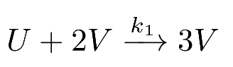
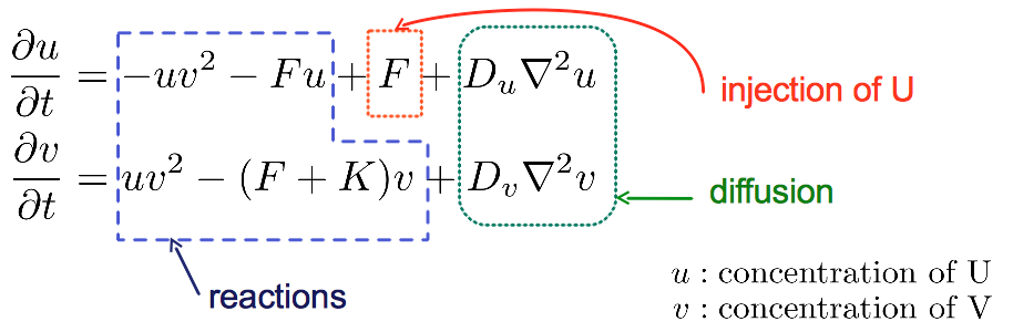
is a famous reaction-diffusion (RD) system where two substances, an activator V and a substrate U, react and diffuse on a virtual plate akin to a Petri Dish. Activator V is an autocatalyst that needs substrate V to replicate itself:
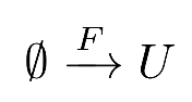
Since it is consumed by the activator V, the substrate U must be constantly replenished from an outside source:
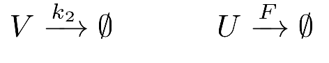
Both chemicals also decay in time:
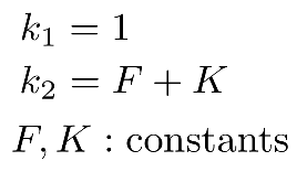
The kinetic coefficients are:
The GrayScott.py example was introduced in PyCellChemistry 2.0 in order to illustrate spatial artificial chemistries. In contrast to other implementations of the Gray-Scott system, here we shall specify only the chemical reactions and other parameters of the system. The ReactionDiffusion.py module from PyCellChemistry takes care of producing the corresponding equations in matrix form, and numerically integrating them. The reaction term of the PDE is produced by applying the law of mass action as it is done for well-mixed systems. The difference now is that we have an extra diffusion term to deal with. Hence ReactionDiffusionSystem is an extension of the ReactionVessel class able to handle two-dimensional grids of chemicals.
The source code of the demo is shown in Figure 2 below. First of all we specify the dimensions of the grid:
        self.gsize = 128
        self.dx = 2.5 / 256
This creates a grid of 128 x 128 cells, each cell representing a space of size dx x dx. This grid has one quarter of the original size 256 x 256 used in [Pearson1993], where it discretized a space of size 2.5 x 2.5 square units of length. We use the same dx value from Pearson in order to reproduce his results as closely as possible, but simulate a reduced portion of the grid, just to make it run faster.
The reactions of the system are then specified:
        reactionstrs = [ "U + 2 V --> 3 V",
                         "      V -->    ",
                         "        --> U  ",
                         "      U -->    "  ]
Since we want to be able to play with the coefficients F and K, they are not predefined in the reaction list reactionstrs but will be specified a bit later.
We then specify the parameters of the system:
        sigma = 4.0
        DU = 2e-5
        DV = DU / sigma
        F = 0.04
        K = 0.06
After that we create an object of class
ReactionDiffusionSystem
which is our PDE integrator, and parse the reactions through it as we did in the Dimer example:
We then set the reaction coefficients of the 2nd, 3rd and 4th reactions (remember that list elements in python are numbered starting from zero, so the first reaction, with list index 0, will keep its default coefficient k=1):
        self.rsys = ReactionDiffusionSystem(self.gsize, self.gsize, self.dx)
        self.rsys.parse(reactionstrs)
        self.rsys.set_coefficient(1, F+K)  # V decays with rate F+K
        self.rsys.set_coefficient(2, F)    # U is injected with rate F
        self.rsys.set_coefficient(3, F)    # U also decays with rate F
After that we set the diffusion coefficients for each chemical:
        self.rsys.set_diffcoef('U', DU)
        self.rsys.set_diffcoef('V', DV)
We then assign colors to each chemical, for visualization purposes:
	self.rsys.set_color( 'U', (0.5, 0, 0) ) # substrate U is dark red
	self.rsys.set_color( 'V', (0, 0, 1) )   # autocatalyst V is blue
The set_color method of ReactionDiffusionSystem takes the color in the form of a tuple (R, G, B) indicating the levels of red, green, and blue (respectively) as floating point numbers between 0 and 1.
Finally we are ready to specify the initial conditions of the system:
        self.rsys.resetAll('U', 0.5)
        initpos = self.gsize/2
        self.rsys.deposit('V', 0.5 * 2, initpos, initpos)
First of all we set the concentration of U to 0.5 over the whole grid using the
resetAll
method.
We then
deposit
an amount of V at the center of the grid, with twice the concentration of U, that is, 0.5 * 2 = 1.0.
We are now done with the initialization part. The
run
method can then be invoked to run the system.
The most important line of
run
is the one that invokes the
integrate
method
to integrate the Gray-Scott PDE numerically with a timestep of size dt
(dt should be sufficiently small: in the case of the Gray-Scott system, the literature says that dt should be smaller than dx ** 2 / (2 * max(DU, DV)).)
The rest of the code in
run
is dedicated to the visualization.
We can watch the results on the screen as an animation, and also save PNG snapshots of the system.
We don't want to fill the filesystem with very similar PNG files, so we write at most n=10 PNGs during the whole simulation, plus one at the beginning with the initial conditions. We invoke the
writepng
method for that.
This will produce a series of files gs0.png, gs1, ..., gs10.png. Each file will contain an image of size 512 x 512 pixels.
Similarly, we don't want to overload the computer with animation rendering of very similar images (actually the concentrations don't change that much from one integration time step dt to the next), so we refresh the animation
(by invoking the
animate
method)
only once every 50 dt's.
As a side note, both
writepng
and
animate
have a transparent option to produce images with a transparent background. This can be useful when there are many spots without chemicals, which would show up in black when transparent is set to False. These empty spots can be displayed as a transparent background instead, when the transparent flag is set. Since in our example we have chemicals everywhere, this option is not very useful here, so it is set to False.
Figure 2: GrayScott.py source code
from ReactionDiffusion import *

class GrayScottDemo():
    def __init__( self ):
        self.gsize = 128
        self.dx = 2.5 / 256
        reactionstrs = [ "U + 2 V --> 3 V",
                         "      V -->    ",
                         "        --> U  ",
                         "      U -->    "  ]
        sigma = 4.0
        DU = 2e-5
        DV = DU / sigma
        F = 0.04
        K = 0.06
        self.rsys = ReactionDiffusionSystem(self.gsize, self.gsize, self.dx)
        self.rsys.parse(reactionstrs)
        self.rsys.set_coefficient(1, F+K)
        self.rsys.set_coefficient(2, F)
        self.rsys.set_coefficient(3, F)
        self.rsys.set_diffcoef('U', DU)
        self.rsys.set_diffcoef('V', DV)
	self.rsys.set_color( 'U', (0.5, 0, 0) )
	self.rsys.set_color( 'V', (0, 0, 1) )
        self.rsys.resetAll('U', 0.5)
        initpos = self.gsize/2
        self.rsys.deposit('V', 0.5 * 2, initpos, initpos)

    def run( self, finalvt=3000.0, dt=0.1 ):
        i = 0
        n = 10
        m = int(finalvt / (dt * n))
        pngsize = 512
        self.rsys.writepng('gs0.png', pngsize, pngsize, transparent=False)
        while (self.rsys.vtime() <= finalvt):
            self.rsys.integrate(dt)
            i += 1
            if (i % m == 0):
                fname = ('gs%d.png' % (i / m) )
                self.rsys.writepng(fname, pngsize, pngsize, transparent=False)
            if (i % 50 == 0):
                self.rsys.animate(sleeptime=0.01, transparent=False)

demo = GrayScottDemo()
demo.run()
   cd pycellchem-2.0/src/RD

   python GrayScott.py
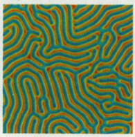
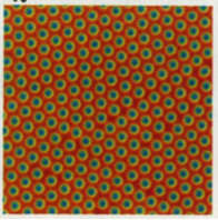
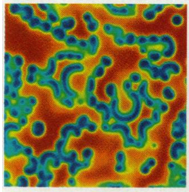
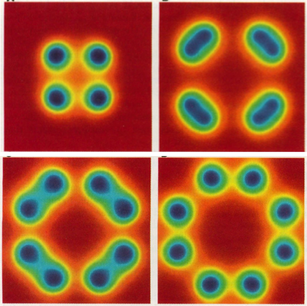
The result should look like this:
Moreover a series of files gs0.png, gs1, ..., gs10.png are generated, which can be visualized by simply clicking on them. The series of PNGs can be combined into a single animated GIF file with the following command from the
ImageMagick
software suite:
convert -delay 50 gs*.png gsanimated.gif
A similar command was used to produce
Figure 3 above.
It is also possible to run this and other RD examples without interactive visualization: it suffices to comment out the animate method and invoke the example as before. You can then rely on writepng to produce periodic snapshots of the grid of chemicals in PNG format.
The implementation of writepng is standalone, that is, it does not rely on any external libraries or modules. This has been achieved thanks to Blender's thumbnailer, which we used as suggested in this post. The full implementation can be found in the module WritePNG.py.
The Gray-Scott system can produce many other interesting patterns. It is only a matter of modifying the parameters of the demo, including the initial conditions. In the example of Figure 3 we started with an accumulation of V on a central spot. Another common initial configuration is a random amount of V all over the grid. Some of these alternative parameters and configurations have been commented out within the source code of the demo. You may want to try them out and see how they work.
You may also want to explore your own parameter ranges, etc. The parameter space for pattern formation has been mapped in [Pearson1993] and then more extensively studied in [Mazin1996]. According to these papers, some conditions for pattern formation are:
Only a very narrow range of F & K combinations lead to patterns (see map in [Pearson1993]). Moreover this range becomes narrower with decreasing sigma (see [Mazin1996] p. 379).
PyCellChemistry 2.0 comes with a few other RD demos:
These demos are very similar to the Gray-Scott demo in their implementation: specify the chemical reactions, rate coefficients, diffusion coefficients, initial conditions, and whether you would like to see an animation on the screen and/or record the results as a series of PNG files. It should be easy to modify these demos and play around with the patterns.
After learning how the examples in the package work, it should be fairly easy to create your own reaction-diffusion system in a very short time. The easiest route to this is of course to modify one of the existing examples to take into account your own reactions and parameters. As a source of inspiration, numerous RD systems have been documented in the literature, see for instance [Meinhardt1982] [Koch1994] [Meinhardt2003].
![]()
Last updated: September 26, 2015, by Lidia Yamamoto