PyCellChemistry: The Chameleons Example

The Chameleons.py example is a simple nonconstructive chemistry inspired by the following puzzle from [Winkler2009a]:

A colony of chameleons includes 20 red, 18 blue, and 16 green individuals. Whenever two chameleons of different color meet, each changes to the third color. Some time passes during which no chameleons are born or die, nor do any enter or leave the colony. Is it possible that at the end of this period all 54 chameleons are the same color?

The answer is "no" for this particular initial configuration [Winkler2009b]. Yet for many other configurations the answer is "yes": it suffices that the difference between the number of chameleons of different colors is a multiple of 3. In practice a "yes" outcome is rare: random encounters between chameleons are dominated by the most frequent ones, just the opposite of the very low number required for the mathematical problem posed here.

It is easy to model this system as an AC. For instance we could simply enumerate all possible reactions explicitly:

        reactionstrs = [
            "red + green --> 2 blue",
            "red + blue  --> 2 green",
            "blue + green --> 2 red"
        ]

However for this particular case we have chosen to implement the same algorithm as the one that appears in our book (page 34) for this example, since it leads to a simple and compact implementation, suitable for an introductory example.

We start by representing each color by a number: red=1, green=2, blue=3. This trick allows us to compute the 3rd color immediately from any 2 different colors:

        color3 = 6 - (color1 + color2)

The core of the code for this example is shown in figure 1. Initially (lines 3-6 of figure 1), a multiset of molecules is created to represent the reacttion vessel, and two populations of N=2700 chameleons of each of the initial colors red and green are injected into the vessel.

After that (lines 7-19 of figure 1), a number niter=12000 of iterations of the following algorithm are executed:

• Two molecules m1 and m2 are drawn at random from the vessel (lines 11-12).
• If they have a different color (line 13), a molecule m3 is produced which is of a 3rd color (line 14), and two copies of m3 are injected into the vessel (line 15).
• If they have the same color (lines 16-18) then the collision is elastic, and the two molecules m1 and m2 return to the vessel without being changed.
• The counts of each molecule type are recorded (printed to the standard output) for subsequent plotting (lines 9 and 19).

Finally, we bootstrap the system by creating an object of class Chameleons, and then run it with the method run (lines 21-22 of figure 1).

 1: from artchem.Multiset import *
 2: class Chameleons:
 3:    def __init__( self, N=2700 ):
 4:        self.mset = Multiset()
 5:        self.mset.inject(1, N)
 6:        self.mset.inject(2, N)
 7:    def run( self, niter=12000 ):
 8:        print "time\tR\tG\tB"
 9:        self.trace_mult(0)
10:        for i in range(niter):
11:            m1 = self.mset.expelrnd()
12:            m2 = self.mset.expelrnd()
13:            if (m1 != m2):
14:                m3 = 6 - (m1 + m2)
15:                self.mset.inject(m3, 2)
16:            else:
17:                self.mset.inject(m1)
18:                self.mset.inject(m2)
19:            self.trace_mult(i+1)
20: if __name__ == '__main__':
21:    chams = Chameleons()
22:    chams.run()

(Footnote: line 20 ensures that the code in the file Chameleons.py is only executed when invoked directly as a script, not when it is included from another script; this check is especially important to avoid Python from executing this code when generating the HTML reference documentation automatically with pydoc)

Running the example

You can now run this program by invoking it from Python. From a Unix command line shell:

cd pycellchem-2.0/src
python Chameleons.py > chameleon.gr

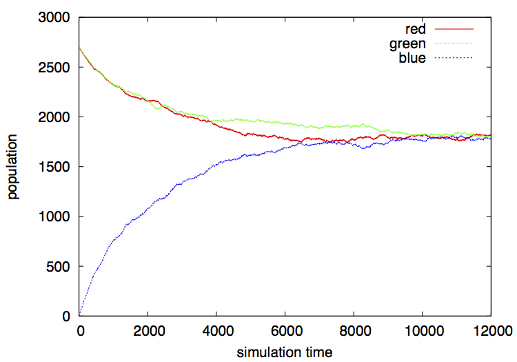
This will produce a tab-separated file chameleon.gr with the population numbers of red, green and blue chameleons over time. You will see that at some point in time the system reaches an equilibrium in which the number of chameleons of each color remains stable (figure 2).

Since this is a stochastic simulation, every time you run the system you will get a different output, however these outputs will look quite similar in general, always converging to an equilibrium where the population numbers remain roughly unchanged.

Running the example from a shell script

Another way to run this example is to invoke the chameleons.sh shell script found in the src/scripts folder:

cd pycellchem-2.0/src
./scripts/chameleons.sh

Note that the chameleons.sh script is located in the src/scripts folder, but it must be involked from the src/ folder where the examples are located, such that the corresponding python source files can be correctly found.

This script invokes Python as before, and plots the output file chameleon.gr using gnuplot. A file chameleon.eps is produced: it depicts the populations of the chameleons of different colors over time. This file can be visualized by simply clicking on it, or from the command line on MacOS with

open chameleon.eps

and on Linux with various tools such as gv or gimp.

The result is:

Modifying the example

Something simple to do is to change the initial population (number of individuals and colors) and see what happens: Does it converge as before? Compare the stochastic fluctuations observed under smaller versus larger total populations. How smaller can you make the total population and still observe some convergence to a stable state?

You are also invited to solve Winkler's puzzle stated at the beginning of this page, namely to find an initial configuration for which the system converges to a single color
Click here for some solutions to this puzzle.

Another "homework" would be to reimplement this system using ODE integration or Gillepie's SSA as done in the Dimer, DimerStoch, Lotka and other examples. Which implementation variant runs faster/slower and under which conditions?

Last updated: July 14, 2015, by Lidia Yamamoto